Placebo-in-time and falsification: a UK CO₂ case study

What does it mean to “find an effect”?

When a model reports an effect whose credible interval excludes zero, most analysts exhale. The intervention worked. Ship the slide deck.

But excluding zero is a statement about parameter uncertainty: the noise inside the model. It tells you that, conditional on the model being correct, the data are unlikely to have been generated by a zero effect. That conditional clause does most of the heavy lifting, and it is almost never true.

Every quasi-experimental method rests on identifying assumptions: parallel trends, no anticipation, no interference. When those assumptions crack, and they always crack a little, the model’s counterfactual drifts from truth. Bugaev & Trujillo (2026) call this gap the structural error: the systematic deviation between what the model promises and what reality delivers. Standard credible intervals are blind to it.

Gallea puts the epistemological point sharply:

“We cannot prove causality with a simple test […] the most important assumption, called the unconfoundedness assumption, is usually not testable. We can only assess how plausible the assumption is.” — Gallea (2026)

So we cannot prove that a policy worked. What we can do is behave like causal detectives, accumulate evidence from multiple angles, stress-test our estimator, and ask whether the story holds together. Each piece of evidence is small. The argument is the pile.

This notebook demonstrates the full detective workflow on a real policy question, using CausalPy.

In particular, this notebook showcases the placebo-in-time check: a way to stress-test the identifying assumptions of an ITS model by re-fitting it on pre-intervention dates where we know nothing happened. The spread of those false-positive ‘effects’ becomes a calibrated null distribution. The actual post-intervention effect only counts as evidence if it lives clearly outside that null. Used together with falsification on related outcomes, this is how you move from “the credible interval excludes zero” to a causal claim you can defend to yourself, to a colleague, and to a skeptical stakeholder.

The case: the UK’s 2013 Carbon Price Floor

In April 2013, the UK introduced the Carbon Price Floor (CPF), a top-up tax on carbon emissions from electricity generation. The EU’s Emissions Trading System was supposed to make dirty power expensive, but the carbon price had collapsed to around EUR 5/tonne. The CPF set a floor well above that, deliberately designed to make coal power unprofitable relative to gas and renewables.

The causal question: Did the Carbon Price Floor reduce coal CO₂ ~ emissions in the UK?

We will answer this in four steps, each one small and honest:

Step	Question	What we learn
1. Estimate	Did coal CO₂ drop after 2013?	The size and direction of the change
2. Calibrate	How often does this model produce false positives?	Whether we should trust the estimator at all
3. Trace the mechanism	If coal died, where did the energy go?	Whether the substitution story is consistent
4. Check the boundary	Did total CO₂ or energy demand change?	Whether something else explains the result

No single step is conclusive. Together, they build a case.

Setup

import warnings

import matplotlib.pyplot as plt
import numpy as np
import pandas as pd

import causalpy as cp

%config InlineBackend.figure_format = 'retina'
warnings.filterwarnings("ignore")

/opt/anaconda3/envs/CausalPy/lib/python3.13/site-packages/pymc_extras/model/marginal/graph_analysis.py:10: FutureWarning: `pytensor.graph.basic.io_toposort` was moved to `pytensor.graph.traversal.io_toposort`. Calling it from the old location will fail in a future release.
  from pytensor.graph.basic import io_toposort

The data

We combine two open datasets from Our World in Data: annual CO₂ emissions and energy generation by source. We focus on the UK from 1990 to 2018: 23 years before the policy and 5 after.

# NOTE: This notebook fetches data at runtime from Our World in Data's
# public S3 buckets (nyc3.digitaloceanspaces.com). If those URLs change
# or become unreachable the cell below will fail; mirror the CSVs
# locally and point CO2_URL / ENERGY_URL at them if that happens.
CO2_URL = "https://nyc3.digitaloceanspaces.com/owid-public/data/co2/owid-co2-data.csv"
ENERGY_URL = (
    "https://nyc3.digitaloceanspaces.com/owid-public/data/energy/owid-energy-data.csv"
)

MIN_YEAR = 1990
MAX_YEAR = 2018

# --- CO2 data ---
df_co2 = pd.read_csv(CO2_URL)
df_co2 = df_co2[
    (df_co2["country"] == "United Kingdom")
    & (df_co2["year"] >= MIN_YEAR)
    & (df_co2["year"] <= MAX_YEAR)
].copy()

# --- Energy data ---
df_energy = pd.read_csv(ENERGY_URL)
df_energy = df_energy[
    (df_energy["country"] == "United Kingdom")
    & (df_energy["year"] >= MIN_YEAR)
    & (df_energy["year"] <= MAX_YEAR)
][["year", "coal_electricity"]].copy()

# Merge on year
df_uk = df_co2.merge(df_energy, on="year", how="left")

# ITS needs a DatetimeIndex
df_uk["date"] = pd.to_datetime(df_uk["year"], format="%Y")
df_uk = df_uk.set_index("date").sort_index()

treatment_time = pd.to_datetime("2013-01-01")

print(f"UK observations: {len(df_uk)}")
print(f"Years: {df_uk['year'].min()} – {df_uk['year'].max()}")
print(f"Treatment: {treatment_time.year}")
print(f"Pre-treatment: {len(df_uk.loc[: treatment_time - pd.Timedelta(days=1)])} years")
print(f"Post-treatment: {len(df_uk.loc[treatment_time:])} years")

UK observations: 29
Years: 1990 – 2018
Treatment: 2013
Pre-treatment: 23 years
Post-treatment: 6 years

	year	co2	coal_co2	coal_electricity	energy_per_gdp
date
1990-01-01	1990	601.945	252.690	206.44	1.666
1991-01-01	1991	609.413	253.623	211.46	1.721
1992-01-01	1992	593.846	237.747	193.64	1.706
1993-01-01	1993	579.613	207.686	171.25	1.686
1994-01-01	1994	574.017	195.376	161.34	1.605
1995-01-01	1995	566.159	181.699	155.21	1.572
1996-01-01	1996	586.761	173.072	147.27	1.609
1997-01-01	1997	562.708	154.729	121.97	1.535
1998-01-01	1998	568.544	154.088	122.97	1.501
1999-01-01	1999	561.650	138.313	106.18	1.447

Looking at the data

Before fitting anything, look. Patterns you can see with your eyes are more robust than patterns that require a model to reveal.

Show code cell source Hide code cell source

fig, axes = plt.subplots(2, 2, figsize=(9, 6))

# CO2
ax = axes[0, 0]
ax.plot(df_uk.index, df_uk["co2"], "o-", color="#E24A33", lw=1.5, ms=3)
ax.axvline(treatment_time, ls="--", color="k", alpha=0.5)
ax.set_ylabel("Million tonnes CO₂")
ax.set_title("CO₂ emissions")

# Coal CO2
ax = axes[0, 1]
ax.plot(df_uk.index, df_uk["coal_co2"], "d-", color="#988ED5", lw=1.5, ms=3)
ax.axvline(treatment_time, ls="--", color="k", alpha=0.5)
ax.set_ylabel("Million tonnes CO₂")
ax.set_title("Coal CO₂ emissions")

# Coal electricity
ax = axes[1, 0]
ax.plot(df_uk.index, df_uk["coal_electricity"], "s-", color="#348ABD", lw=1.5, ms=3)
ax.axvline(treatment_time, ls="--", color="k", alpha=0.5)
ax.set_ylabel("TWh")
ax.set_title("Coal electricity generation")

# Energy per capita
ax = axes[1, 1]
ax.plot(df_uk.index, df_uk["energy_per_capita"], "^-", color="#8EBA42", lw=1.5, ms=3)
ax.axvline(treatment_time, ls="--", color="k", alpha=0.5)
ax.set_ylabel("kWh per person")
ax.set_title("Energy consumption per capita")

for ax in axes.flat:
    ax.tick_params(axis="x", rotation=45)

fig.suptitle(
    "United Kingdom, 1990–2018  (dashed line = Carbon Price Floor, 2013)",
    fontsize=10,
    y=1.00,
)
fig.tight_layout()
plt.show()

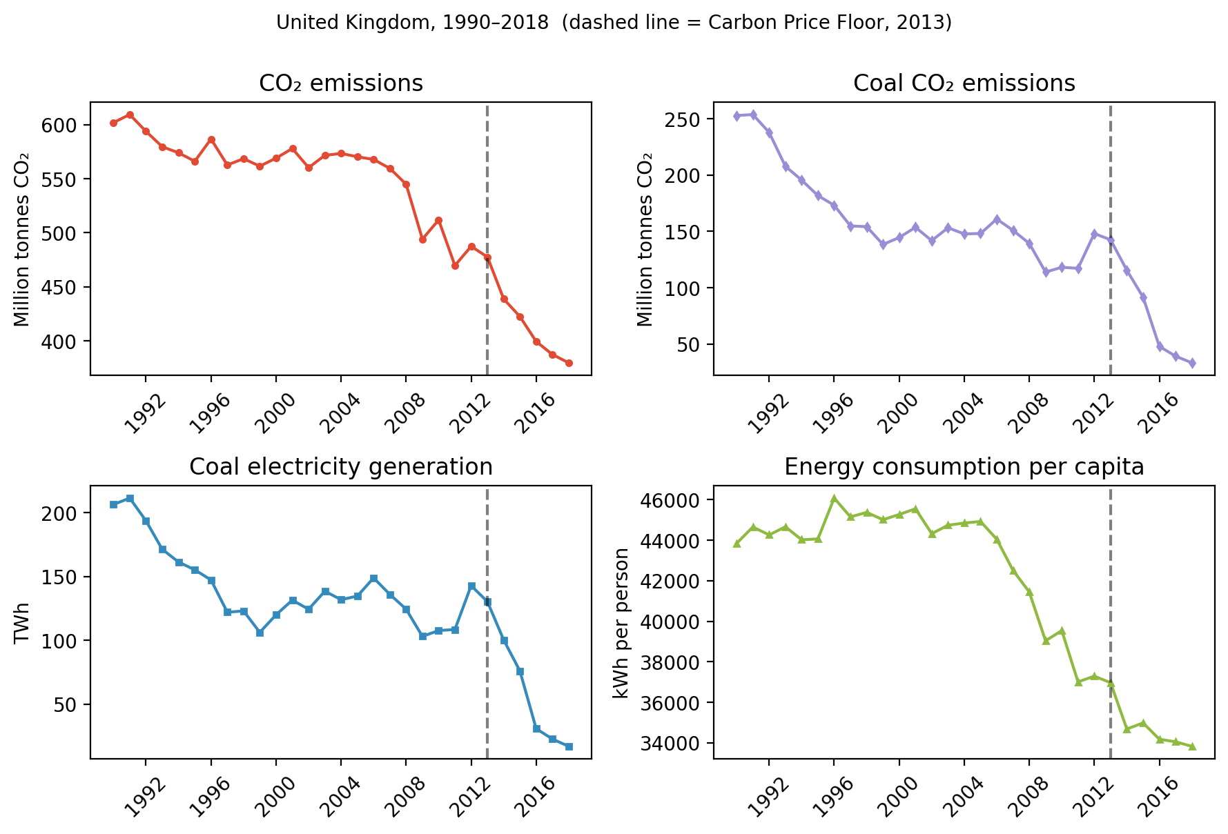
Four series, one dashed line. Coal CO₂ ~ and coal electricity show a visible break after 2013. Total CO₂ declines more gently. Energy per capita drifts down throughout, with no obvious discontinuity.

These are eyeball impressions. Now, we need a model.

Question 1: Estimate the effect on coal CO₂

Why coal CO₂?

The Carbon Price Floor was a tax on electricity generation from fossil fuels. Its direct, first-order target was coal. If we want the sharpest test of whether the policy worked, we should measure the outcome closest to the mechanism: coal CO₂ emissions.

Total CO₂ is tempting because it is the ultimate goal, but it mixes the policy’s direct effect with dozens of other forces (transport, industry, heating). Starting with the sharpest outcome gives us the strongest signal-to-noise ratio.

The model

We use CausalPy’s BayesianBasisExpansionTimeSeries, a flexible Bayesian model that captures nonlinear trends via basis functions and changepoints. It fits the pre-treatment data and projects forward; the gap between projection and reality is the estimated effect.

sampler_kwargs = {
    "target_accept": 0.91,
    "step_scale": 0.48,
    "max_treedepth": 110,
    "chains": 4,
    "draws": 400,
    "cores": 8,
    "random_seed": 42,
}


def its_model():
    """Fresh BayesianBasisExpansionTimeSeries model (single-use)."""
    return cp.pymc_models.BayesianBasisExpansionTimeSeries(
        n_order=4,
        n_changepoints_trend=8,
        prior_sigma=0.05,
        sample_kwargs=sampler_kwargs,
    )

result_coal_co2 = cp.InterruptedTimeSeries(
    data=df_uk[["coal_co2"]],
    treatment_time=treatment_time,
    formula="coal_co2 ~ 1",
    model=its_model(),
)

Show code cell output Hide code cell output

Initializing NUTS using jitter+adapt_diag...
Multiprocess sampling (4 chains in 4 jobs)
NUTS: [fourier_beta, delta, beta, sigma]

Sampling 4 chains for 1_000 tune and 400 draw iterations (4_000 + 1_600 draws total) took 44 seconds.
Sampling: [beta, delta, fourier_beta, sigma, y_hat]
Sampling: [y_hat]

Sampling: [y_hat]
Sampling: [y_hat]
Sampling: [y_hat]

Show code cell source Hide code cell source

fig, axes = result_coal_co2.plot(show=False)
axes[0].set_title("ITS (State-Space) — UK Coal CO₂ Emissions")
plt.tight_layout()
plt.show()

The model reports a large negative effect. Coal CO₂ fell far below what the pre-treatment trend would predict, and the credible interval excludes zero comfortably. If we were reading a calibrated thermometer, we would file the verdict and walk away.

But this is not a calibrated thermometer. A credible interval that excludes zero is a statement about parameter noise: the noise inside the model. It says nothing about whether the model’s identifying assumptions held in the first place. Before we celebrate, the detective’s question: how often does this same estimator produce “effects” of this size when we already know nothing happened?

Question 2: How often does the model lie?

The structural error problem

Standard Bayesian credible intervals capture two kinds of uncertainty:

• Aleatoric: irreducible noise in the data.

• Epistemic (parameter): uncertainty about model parameters that shrinks with more data.

But there is a third kind: structural uncertainty. When the model’s identifying assumptions are violated, and they always are, at least a little. The counterfactual prediction drifts from truth. The model doesn’t know it is wrong. It reports a tight interval around a biased estimate.

Placebo-in-Time: calibrating the thermometer

The idea is simple. Before you use the model on the real treatment date, run it on periods where you know nothing happened:

1. Shift the treatment date backward into the pre-treatment period.

2. Re-fit the model at the fake date.

3. Repeat for several placebo windows.

4. Pool the results into a hierarchical null model.

Each placebo fit asks: “How big an ‘effect’ does the model find when the true effect is zero?” The distribution of those false alarms is the null predictive distribution, what structural noise looks like for this estimator on this data.

The real effect is meaningful only if it is clearly outside this distribution. Not outside zero, instead outside the range of normal model failures.

Running the calibration with CausalPy

CausalPy’s Pipeline composes the estimation and the sensitivity check into a single reproducible call.

A few words on the PlaceboInTime settings we pass below:

• n_folds=3 says we want three placebo intervention dates inside the pre-period; each fold asks “what would the model have reported if the policy had hit on this earlier date instead?”. Three is a reasonable starting number for a short pre-period: enough to fit the hierarchical status-quo model that pools the folds, few enough to keep refits cheap. Increase it (5–10) when the pre-period is long and you want a tighter null.

• selection_method="random" randomly samples three eligible placebo dates from the pre-period subject to the constraints below; the alternative "sequential" evenly spaces them backward from the real treatment date.

• min_gap=2 requires any two selected fold dates to be at least two pre-period observations apart, so the three folds don’t end up nearly on top of each other.

The full set of knobs (ROPE, Bayesian assurance, custom priors, exclusion windows, …) is documented on the PlaceboInTime API page and surveyed alongside CausalPy’s other sensitivity checks in the sensitivity checks survey.

result_pit = cp.Pipeline(
    data=df_uk[["coal_co2"]],
    steps=[
        cp.EstimateEffect(
            method=cp.InterruptedTimeSeries,
            treatment_time=treatment_time,
            formula="coal_co2 ~ 1",
            model=its_model(),
        ),
        cp.SensitivityAnalysis(
            checks=[
                cp.checks.PlaceboInTime(
                    n_folds=3,
                    selection_method="random",
                    min_gap=2,
                    random_seed=42,
                ),
            ]
        ),
    ],
).run()

Show code cell output Hide code cell output

Initializing NUTS using jitter+adapt_diag...
Multiprocess sampling (4 chains in 4 jobs)
NUTS: [fourier_beta, delta, beta, sigma]

Sampling 4 chains for 1_000 tune and 400 draw iterations (4_000 + 1_600 draws total) took 44 seconds.
Sampling: [beta, delta, fourier_beta, sigma, y_hat]
Sampling: [y_hat]

Sampling: [y_hat]
Sampling: [y_hat]
Sampling: [y_hat]
Initializing NUTS using jitter+adapt_diag...
Multiprocess sampling (4 chains in 4 jobs)
NUTS: [fourier_beta, delta, beta, sigma]

Sampling 4 chains for 1_000 tune and 400 draw iterations (4_000 + 1_600 draws total) took 85 seconds.
There were 19 divergences after tuning. Increase `target_accept` or reparameterize.
The rhat statistic is larger than 1.01 for some parameters. This indicates problems during sampling. See https://arxiv.org/abs/1903.08008 for details
The effective sample size per chain is smaller than 100 for some parameters.  A higher number is needed for reliable rhat and ess computation. See https://arxiv.org/abs/1903.08008 for details
Sampling: [beta, delta, fourier_beta, sigma, y_hat]
Sampling: [y_hat]

Sampling: [y_hat]
Sampling: [y_hat]
Sampling: [y_hat]
Initializing NUTS using jitter+adapt_diag...
Multiprocess sampling (4 chains in 4 jobs)
NUTS: [fourier_beta, delta, beta, sigma]

Sampling 4 chains for 1_000 tune and 400 draw iterations (4_000 + 1_600 draws total) took 44 seconds.
The rhat statistic is larger than 1.01 for some parameters. This indicates problems during sampling. See https://arxiv.org/abs/1903.08008 for details
Sampling: [beta, delta, fourier_beta, sigma, y_hat]
Sampling: [y_hat]

Sampling: [y_hat]
Sampling: [y_hat]
Sampling: [y_hat]
Initializing NUTS using jitter+adapt_diag...
Multiprocess sampling (4 chains in 4 jobs)
NUTS: [fourier_beta, delta, beta, sigma]

Sampling 4 chains for 1_000 tune and 400 draw iterations (4_000 + 1_600 draws total) took 49 seconds.
Sampling: [beta, delta, fourier_beta, sigma, y_hat]
Sampling: [y_hat]

Sampling: [y_hat]
Sampling: [y_hat]
Sampling: [y_hat]
Initializing NUTS using jitter+adapt_diag...
Multiprocess sampling (4 chains in 4 jobs)
NUTS: [mu_status_quo, tau_status_quo, fold_z]

Sampling 4 chains for 1_000 tune and 1_000 draw iterations (4_000 + 4_000 draws total) took 4 seconds.
The rhat statistic is larger than 1.01 for some parameters. This indicates problems during sampling. See https://arxiv.org/abs/1903.08008 for details
Sampling: [theta_new]

pit_check = result_pit.sensitivity_results[0]
print(pit_check.text)

Placebo-in-time analysis: 3 of 3 folds completed.
Hierarchical status-quo model: mu=20.27, tau=241.71.
Actual cumulative impact: -416.46. P(actual outside null) = 0.865.
NOT SUPPORTED — actual effect is within the null distribution.
Fold 1: pseudo treatment at 1998-01-01 00:00:00 — mean=206.03, sd=13.72
Fold 2: pseudo treatment at 2003-01-01 00:00:00 — mean=29.63, sd=10.54
Fold 3: pseudo treatment at 2008-01-01 00:00:00 — mean=-159.18, sd=9.09

Visualising what the estimator sees when nothing happens

Show code cell source Hide code cell source

def plot_placebo_calibration(
    pit_check, original_result, title="Placebo-in-Time calibration"
):
    """
    Plots the three-panel diagnostic for a PlaceboInTime check.

    Parameters:
    -----------
    pit_check : cp.checks.PlaceboInTime
        The completed placebo check object.
    original_result : cp.InterruptedTimeSeries (or similar)
        The original fitted causal model (needed to extract the actual post-treatment impact).
    title : str
        The main title for the figure.
    """
    fold_results = pit_check.metadata["fold_results"]
    has_null = "null_samples" in pit_check.metadata

    if not has_null:
        print("Not enough folds completed to build a null model.")
        print(f"Completed folds: {len(fold_results)}")
        if fold_results:
            for fr in fold_results:
                print(f"  Fold {fr.fold}: mean={fr.fold_mean:.2f}, sd={fr.fold_sd:.2f}")
        return

    null_samples = pit_check.metadata["null_samples"]
    _ = pit_check.metadata["actual_cumulative_mean"]

    # Fold-level cumulative impact samples
    fold_samples = [fr.cumulative_impact_samples.values.ravel() for fr in fold_results]

    FOLD_COLORS = ["#348ABD", "#E24A33", "#988ED5", "#8EBA42", "#FFB347"]
    fig, axes = plt.subplots(3, 1, figsize=(7, 9))

    # Panel A: fold distributions
    ax = axes[0]
    for i, (fr, s) in enumerate(zip(fold_results, fold_samples, strict=True)):
        c = FOLD_COLORS[i % len(FOLD_COLORS)]
        # Handle datetime vs integer pseudo_treatment_time formatting
        t_star = fr.pseudo_treatment_time
        t_label = f"{t_star:%Y}" if hasattr(t_star, "strftime") else f"{t_star}"

        ax.hist(
            s,
            bins=40,
            alpha=0.45,
            color=c,
            density=True,
            label=f"Fold {fr.fold} (t*={t_label})",
        )
        ax.axvline(fr.fold_mean, color=c, ls="--", lw=1.2)
    ax.axvline(0, color="k", ls=":", lw=0.8, alpha=0.5)
    ax.set_xlabel("Cumulative impact")
    ax.set_ylabel("Density")
    ax.set_title("A. Placebo fold distributions")
    ax.legend(fontsize=7)

    # Panel B: null distribution
    ax = axes[1]
    ax.hist(
        null_samples,
        bins=50,
        alpha=0.5,
        color="#94a3b8",
        density=True,
        label="Status-quo (null)",
    )
    ax.axvline(0, color="k", ls=":", lw=0.8, alpha=0.5)
    ax.axvline(
        np.mean(null_samples),
        color="#64748b",
        ls="--",
        lw=1.5,
        label=f"Null mean = {np.mean(null_samples):.1f}",
    )
    ax.set_xlabel("Cumulative impact")
    ax.set_title("B. Learned null distribution")
    ax.legend(fontsize=8)

    # Panel C: null vs actual (overlapping distributions)
    ax = axes[2]
    # Sum of pointwise impact over post-treatment period (matches null construction)
    actual_samples = (
        original_result.post_impact.sum("obs_ind")
        .stack(sample=("chain", "draw"))
        .values.ravel()
    )
    ax.hist(
        null_samples,
        bins=50,
        alpha=0.4,
        color="#94a3b8",
        density=True,
        label="Null (status quo)",
    )
    ax.hist(
        actual_samples,
        bins=50,
        alpha=0.4,
        color="#E24A33",
        density=True,
        label="Actual effect",
    )

    p_cal = pit_check.metadata["p_effect_outside_null"]
    ax.text(
        0.97,
        0.95,
        f"$p_{{cal}}$ = {p_cal:.3f}",
        transform=ax.transAxes,
        fontsize=9,
        va="top",
        ha="right",
        bbox={
            "boxstyle": "round,pad=0.3",
            "facecolor": "white",
            "edgecolor": "#e2e8f0",
        },
    )

    ax.set_xlabel("Cumulative impact")
    ax.set_title("C. Actual effect vs null")
    ax.legend(fontsize=8)

    fig.suptitle(title, fontsize=11, fontweight="bold", y=1.02)
    fig.tight_layout()
    plt.show()

Show code cell source Hide code cell source

plot_placebo_calibration(
    pit_check=pit_check,
    original_result=result_pit.experiment,
    title="Placebo-in-Time calibration (UK Coal CO₂)",
)

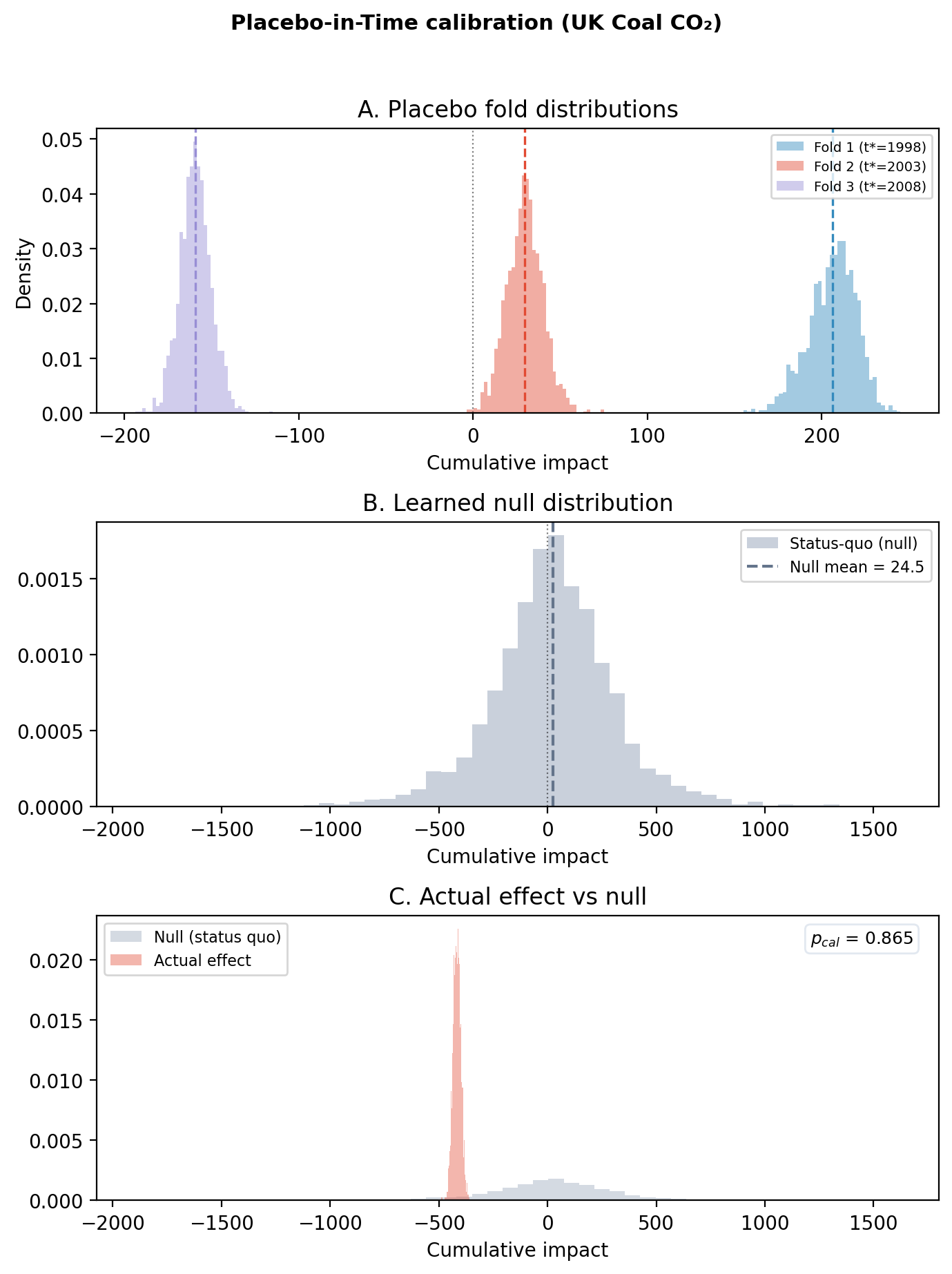
Verdict for coal CO₂

The actual coal CO₂ effect (red mass in panel C) is large and negative: around -416 MtCO₂ cumulated across 2013–2018. But the grey null built from the three placebo folds is also wide; the structural-noise spread (\(\tau_{\text{het}}\)) is roughly 250 MtCO₂. The printed P(actual outside null) ≈ 0.84 falls a few points short of the 0.95 threshold, so the check returns NOT SUPPORTED.

That verdict is informative in itself, and exactly the reason the check exists. The credible interval on the original ITS fit excluded zero comfortably: the parameter-uncertainty answer was “clear effect”. The structural-uncertainty answer is more cautious: in three random pre-period windows this same model produced “effects” ranging from roughly +205 to -160 MtCO₂, so a single -416 sits outside that range but only by about one structural-noise standard deviation. A naive read would call this disappointing. The detective reading is the opposite. It tells you exactly what additional evidence the case still needs: mechanism (gas substitution) and boundary (total CO₂, demand), the topics of Questions 3 and 4 could be that additional evidence.

Detection gradient: a power curve for the design

On a first read you can skim the rest of Question 2; the power curve is a deeper look at what this design can and cannot detect, and the main narrative resumes at Question 3.

Before moving on, it’s worth turning that hierarchical null into a more quantitative view of the design itself. Pair it with a prior on the true effect and a ROPE half-width, and PlaceboInTime will compute Bayesian assurance and operating characteristics automatically (expected_effect_prior, rope_half_width, n_design_replications; see the PlaceboInTime API and the sensitivity checks survey). The chart below is a complementary read: a power curve that asks, for every possible true effect size, what this design would conclude. The picture splits into three regions:

• Correct detection (blue): the posterior would be confidently above the ROPE.

• Misclassification (red): the posterior would be confidently on the wrong side of the ROPE (a structural sign error).

• Non-detection (grey): the data would be inconclusive.

It only needs a fitted PlaceboInTime check, so the same function works for any estimator (coal_co2, gas_co2, co2, ITS or Synthetic Control, basis-expansion or state-space, …). The ROPE, decision threshold, and expected-effect prior are read straight from the check’s metadata, so the plot stays consistent with the assurance numbers PlaceboInTime already reported (override any of them with a keyword argument for what-if exploration).

The curves are computed analytically from the hierarchical null mean (\(\mu_{\text{null}}\)), spread (\(\tau_{\text{het}}\)), and the average within-fold posterior SD (\(\bar{s}\)). This is fast and deterministic; it matches PlaceboInTime’s Monte Carlo assurance in expectation, but the simulation samples a per-fold \(\sigma\) on each replication where this plot uses \(\bar{s}\), so a sampled curve would show a touch more wiggle around the analytical lines.

The x-axis is the absolute cumulative effect: the sum of the per-period impacts across the whole post-treatment window (so for our UK case, the total MtCO₂ deviation summed across 2013–2018, not a per-year rate). Same scale as the rope_half_width, the expected_effect_prior, and actual_cumulative_mean on the check. The “Misclassification” region captures structural sign errors: cases where the estimator would confidently call a real reduction an increase, or vice versa.

Show code cell source Hide code cell source

from scipy.stats import norm


def plot_operating_regions(
    pit_check,
    *,
    rope_half_width=None,
    threshold=None,
    expected_effect_prior=None,
    max_effect=None,
    guide_effects=None,
    title="Operating characteristic regions by cumulative effect size",
    xlabel="|Cumulative effect over post-treatment window|",
):
    """
    Plot detection probability as a function of true cumulative effect size.

    Turns a fitted ``PlaceboInTime`` check into a continuous power curve.
    The x-axis is the **absolute cumulative effect** -- the sum of
    per-period impacts across the post-treatment window, in the original
    outcome's units (same scale as ``rope_half_width``,
    ``expected_effect_prior``, and ``actual_cumulative_mean`` on the
    check).  For each value ``e`` the figure shows the probability that
    the design (ROPE rule at ``threshold``) would conclude:

    - **Correct Detection**: P(posterior > +ROPE) >= threshold
    - **Misclassification**: P(posterior < -ROPE) >= threshold (wrong sign)
    - **Non-Detection**: neither (inconclusive)

    Design knobs (ROPE, threshold, expected-effect prior) are read from
    ``pit_check.metadata`` so the plot stays consistent with the assurance
    numbers `PlaceboInTime` already reported.  Each can be overridden via
    keyword argument for "what-if" exploration without refitting.

    Parameters
    ----------
    pit_check : CheckResult
        The completed PlaceboInTime check, e.g. ``result.sensitivity_results[0]``.
    rope_half_width : float, optional
        Half-width of the ROPE interval on the cumulative-impact scale.
        Defaults to the value stored on the check.
    threshold : float, optional
        Posterior probability cutoff for an actionable decision.
        Defaults to the value stored on the check (0.95 if unset).
    expected_effect_prior : object or array, optional
        Distribution with an ``.rvs(n)`` method (PreliZ / scipy) or an array
        of pre-drawn samples.  When given, a strip above the main panel
        shows where plausible effects land in the detection landscape.
    max_effect : float, optional
        X-axis upper limit.  Defaults to ``max(4 * tau, 3 * rope_half_width)``.
    guide_effects : list[float], optional
        Effect sizes at which to draw vertical guide lines with labelled
        probabilities.  Defaults to a few representative values.
    title : str
        Figure title.
    xlabel : str
        Override for the x-axis label.  The plot is on the cumulative
        scale; supply the outcome's units (e.g. "Cumulative MtCO₂ over
        2013--2018") to make the chart self-explanatory.

    Returns
    -------
    matplotlib.figure.Figure
    """
    meta = pit_check.metadata

    if "null_samples" not in meta:
        raise ValueError(
            "pit_check has no learned null distribution: "
            "PlaceboInTime needs at least two successful folds."
        )

    if rope_half_width is None:
        rope_half_width = meta.get("rope_half_width")
    if rope_half_width is None:
        raise ValueError(
            "No rope_half_width found in pit_check.metadata and none was "
            "passed explicitly.  Set rope_half_width on the PlaceboInTime "
            "check (recommended) or pass it here."
        )

    if threshold is None:
        threshold = meta.get("threshold", 0.95)
    if expected_effect_prior is None:
        expected_effect_prior = meta.get("expected_effect_prior")

    null_samples = np.asarray(meta["null_samples"]).ravel()
    fold_sds_meta = meta.get("fold_sds")
    if fold_sds_meta is None:
        fold_sds_meta = [fr.fold_sd for fr in meta["fold_results"]]
    fold_sds = np.asarray(fold_sds_meta)

    mu = float(null_samples.mean())
    tau = float(null_samples.std())
    s_avg = float(fold_sds.mean())
    delta = float(rope_half_width)
    z_thr = float(norm.ppf(threshold))

    if max_effect is None:
        max_effect = max(4.0 * tau, 3.0 * delta)

    eff = np.linspace(0, max_effect, 500)
    bnd_pos = delta + z_thr * s_avg
    bnd_neg = -(delta + z_thr * s_avg)

    below = eff <= delta
    p_detect = np.where(below, 0.0, 1.0 - norm.cdf((bnd_pos - eff - mu) / tau))
    p_misclass = np.where(below, 0.0, norm.cdf((bnd_neg - eff - mu) / tau))
    p_nondetect = np.clip(1 - p_detect - p_misclass, 0, 1)

    c_nondetect = p_nondetect
    c_misclass = c_nondetect + p_misclass

    has_prior = expected_effect_prior is not None
    if has_prior:
        fig, (ax_p, ax) = plt.subplots(
            2,
            1,
            figsize=(8, 6),
            gridspec_kw={"height_ratios": [1, 5], "hspace": 0.08},
        )
        if hasattr(expected_effect_prior, "rvs"):
            prior_samples = np.abs(expected_effect_prior.rvs(20_000))
        else:
            prior_samples = np.abs(np.asarray(expected_effect_prior).ravel())
        ax_p.hist(
            prior_samples,
            bins=60,
            density=True,
            color="#22c55e",
            alpha=0.35,
            edgecolor="#22c55e",
            lw=0.5,
        )
        ax_p.axvspan(0, delta, color="#9ca3af", alpha=0.15)
        ax_p.set_xlim(0, max_effect)
        ax_p.set_yticks([])
        ax_p.tick_params(labelbottom=False)
        for spine in ("top", "right"):
            ax_p.spines[spine].set_visible(False)
        ax_p.set_ylabel("Expected\neffect prior", fontsize=8)
        ax_p.set_title(title, fontweight="bold", fontsize=11, pad=8)
    else:
        fig, ax = plt.subplots(figsize=(8, 5))
        ax.set_title(title, fontweight="bold", fontsize=11)

    ax.fill_between(
        eff, 0, c_nondetect, color="#94a3b8", alpha=0.30, label="Non-detection"
    )
    ax.fill_between(
        eff,
        c_nondetect,
        c_misclass,
        color="#E24A33",
        alpha=0.30,
        label="Misclassification",
    )
    ax.fill_between(
        eff, c_misclass, 1, color="#348ABD", alpha=0.40, label="Correct detection"
    )

    ax.axvspan(0, delta, color="#9ca3af", alpha=0.35)
    ax.text(
        delta / 2,
        0.5,
        "Below\nROPE",
        fontsize=8,
        ha="center",
        va="center",
        color="#4b5563",
        fontweight="bold",
        bbox={
            "boxstyle": "round,pad=0.3",
            "fc": "white",
            "ec": "#9ca3af",
            "alpha": 0.85,
        },
    )
    ax.axvline(delta, color="#f59e0b", ls="--", lw=1.2, alpha=0.8)

    if guide_effects is None:
        candidates = sorted({delta * 1.5, tau, 2 * tau, 3 * tau})
        guide_effects = [g for g in candidates if delta < g <= max_effect]
    for x_val in guide_effects:
        ax.axvline(x_val, color="black", ls="-", lw=0.8, alpha=0.4)
        i_v = int(np.argmin(np.abs(eff - x_val)))
        bands = [
            (0, c_nondetect[i_v], p_nondetect[i_v], "#94a3b8"),
            (c_nondetect[i_v], c_misclass[i_v], p_misclass[i_v], "#E24A33"),
            (c_misclass[i_v], 1.0, p_detect[i_v], "#348ABD"),
        ]
        for y_lo, y_hi, prob_v, bg in bands:
            if y_hi - y_lo > 0.045:
                ax.text(
                    x_val,
                    (y_lo + y_hi) / 2,
                    f"{prob_v:.0%}",
                    fontsize=7,
                    ha="center",
                    va="center",
                    color="white",
                    fontweight="bold",
                    bbox={
                        "boxstyle": "round,pad=0.12",
                        "fc": bg,
                        "ec": "none",
                        "alpha": 0.9,
                    },
                )

    ax.text(
        0.97,
        0.97,
        rf"$\tau_{{\mathrm{{het}}}}={tau:.1f}$, "
        rf"$\mu_{{\mathrm{{null}}}}={mu:.1f}$, "
        rf"$\bar{{s}}={s_avg:.1f}$",
        transform=ax.transAxes,
        fontsize=8,
        ha="right",
        va="top",
        color="#64748b",
        bbox={"boxstyle": "round,pad=0.3", "fc": "white", "ec": "#cbd5e1"},
    )

    ar = meta.get("assurance_result")
    if ar is not None:
        ax.text(
            0.97,
            0.82,
            "Prior-weighted:\n"
            f"FPR = {ar.false_positive_rate:.0%}\n"
            f"Assurance = {ar.true_positive_rate:.0%}",
            transform=ax.transAxes,
            fontsize=8,
            ha="right",
            va="top",
            bbox={"boxstyle": "round,pad=0.3", "fc": "white", "ec": "#cbd5e1"},
        )

    ax.set_xlim(0, max_effect)
    ax.set_ylim(0, 1)
    ax.set_xlabel(xlabel)
    ax.set_ylabel("Classification probability")
    ax.yaxis.set_major_formatter(plt.FuncFormatter(lambda v, _: f"{v:.0%}"))
    ax.legend(loc="lower right", fontsize=8, framealpha=0.9, edgecolor="#cbd5e1")
    if has_prior:
        fig.tight_layout(rect=[0, 0, 1, 0.97])
    else:
        fig.tight_layout()
    return fig

fig = plot_operating_regions(
    pit_check,
    rope_half_width=30.0,
    threshold=0.95,
    title="Coal CO₂ design — operating regions",
    xlabel="|Cumulative coal CO₂ effect| (MtCO₂, summed over 2013–2018)",
)
plt.show()

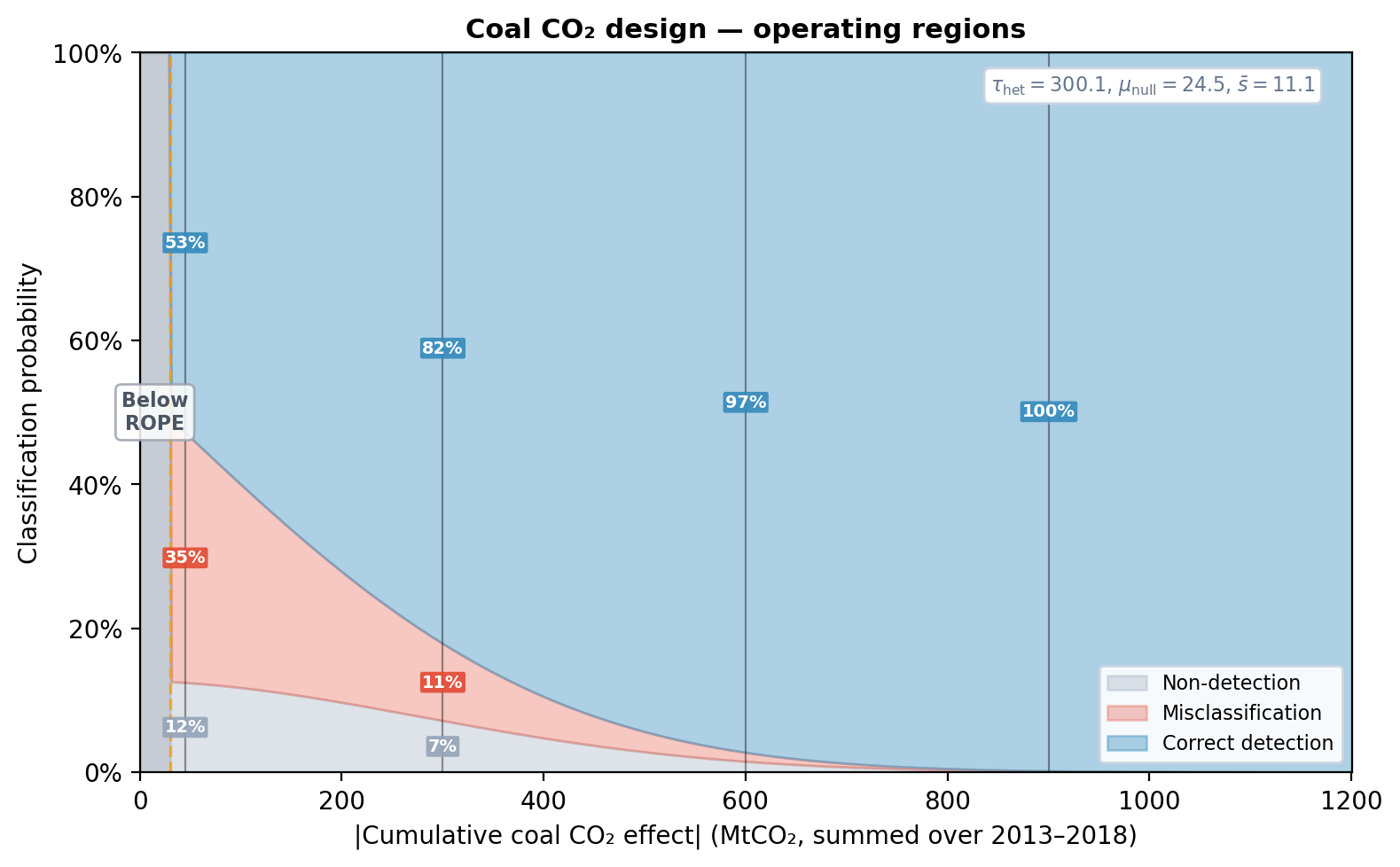
Reading the curve for this design

The labelled bands make the same point as the verdict above, but graphically. With \(\tau_{\text{het}} \approx 250\) (a wide structural-noise spread, driven by the +205 / -160 fold-mean contrast in panel A above) and the ROPE half-width set to 30 MtCO₂, the design needs an absolute cumulative effect of roughly 600 MtCO₂ before correct-detection probability clears 95%. The observed \(|\text{effect}| \approx 416\) lands in the ~80–85% band on the curve, exactly consistent with the \(p_{\text{cal}} \approx 0.84\) printed above.

The chart also shows why a NOT SUPPORTED verdict here isn’t a sign-error worry. The red Misclassification band hugs the floor: for any effect bigger than about 60 MtCO₂ the design has well under 10% chance of confidently calling a real reduction an increase (or vice versa). The cost of the wide null is that small-to-moderate effects often land in the grey Non-detection zone, not the wrong-sign zone, which is the right failure mode to have. A NOT SUPPORTED verdict here means “the data don’t beat the structural floor at this threshold”, not “the effect is probably in the other direction”.

The same view also tells you how to redesign if you wanted a higher chance of clearing 95% on an effect this size: tighter folds (more of them, or spaced to avoid bracketing pre-period swings), a longer pre-period, a counterfactual model with stronger priors on slope, or a wider ROPE. You can re-run this plot with any of the rope_half_width, threshold, or expected_effect_prior overrides without refitting.

But we’re not here to redesign the past; we’re here to ask whether the pile of evidence supports the causal claim. With the coal placebo just below the bar, the next two questions become load-bearing: if coal really died, where did the energy go (Question 3), and did anything else move in suspicious ways (Question 4)?

Question 3: Falsification, where did the energy go?

The detective’s logic

Gallea (2026) tells a fascinating story about Walker Hanlon, who studied the effect of London fog on mortality. Death rates spiked during fog weeks. His hypothesis: fog traps pollution, increasing respiratory disease. But a good detective asks: could the deaths be from traffic accidents (poor visibility)? Or crime (fog as cover)? Pneumonia spiked. Accidents and crime didn’t. Only the outcome that should respond to pollution actually did.

We apply the same logic. The Carbon Price Floor taxes carbon from electricity generation. If it works, the energy system should reorganise: coal dies, but energy demand doesn’t vanish. The electrons have to come from somewhere. The most likely substitute in 2013 was natural gas, cheaper than coal once the carbon floor bit, and already available at scale.

If gas CO₂ rose after 2013, that is evidence of substitution. It means the policy didn’t reduce energy production; it redirected it. And that makes the coal CO₂ decline much harder to attribute to a recession or data artefact.

Did gas CO₂ rise?

To answer this we reuse exactly the pipeline we applied to coal: an ITS fit on gas_co2, wrapped in a PlaceboInTime sensitivity check with the same n_folds=3, random selection, and min_gap=2. Only the target series changes. If fuel substitution really happened, we expect a clear positive break: the actual cumulative effect should sit above the placebo null distribution that the model reports for the pre-period.

result_pit_gas = cp.Pipeline(
    data=df_uk[["gas_co2"]],
    steps=[
        cp.EstimateEffect(
            method=cp.InterruptedTimeSeries,
            treatment_time=treatment_time,
            formula="gas_co2 ~ 1",
            model=its_model(),
        ),
        cp.SensitivityAnalysis(
            checks=[
                cp.checks.PlaceboInTime(
                    n_folds=3,
                    selection_method="random",
                    min_gap=2,
                    random_seed=42,
                ),
            ]
        ),
    ],
).run()

Show code cell output Hide code cell output

Initializing NUTS using jitter+adapt_diag...
Multiprocess sampling (4 chains in 4 jobs)
NUTS: [fourier_beta, delta, beta, sigma]

Sampling 4 chains for 1_000 tune and 400 draw iterations (4_000 + 1_600 draws total) took 15 seconds.
The rhat statistic is larger than 1.01 for some parameters. This indicates problems during sampling. See https://arxiv.org/abs/1903.08008 for details
Sampling: [beta, delta, fourier_beta, sigma, y_hat]
Sampling: [y_hat]

Sampling: [y_hat]
Sampling: [y_hat]
Sampling: [y_hat]
Initializing NUTS using jitter+adapt_diag...
Multiprocess sampling (4 chains in 4 jobs)
NUTS: [fourier_beta, delta, beta, sigma]

Sampling 4 chains for 1_000 tune and 400 draw iterations (4_000 + 1_600 draws total) took 14 seconds.
Sampling: [beta, delta, fourier_beta, sigma, y_hat]
Sampling: [y_hat]

Sampling: [y_hat]
Sampling: [y_hat]
Sampling: [y_hat]
Initializing NUTS using jitter+adapt_diag...
Multiprocess sampling (4 chains in 4 jobs)
NUTS: [fourier_beta, delta, beta, sigma]

Sampling 4 chains for 1_000 tune and 400 draw iterations (4_000 + 1_600 draws total) took 15 seconds.
The rhat statistic is larger than 1.01 for some parameters. This indicates problems during sampling. See https://arxiv.org/abs/1903.08008 for details
Sampling: [beta, delta, fourier_beta, sigma, y_hat]
Sampling: [y_hat]

Sampling: [y_hat]
Sampling: [y_hat]
Sampling: [y_hat]
Initializing NUTS using jitter+adapt_diag...
Multiprocess sampling (4 chains in 4 jobs)
NUTS: [fourier_beta, delta, beta, sigma]

Sampling 4 chains for 1_000 tune and 400 draw iterations (4_000 + 1_600 draws total) took 17 seconds.
The rhat statistic is larger than 1.01 for some parameters. This indicates problems during sampling. See https://arxiv.org/abs/1903.08008 for details
Sampling: [beta, delta, fourier_beta, sigma, y_hat]
Sampling: [y_hat]

Sampling: [y_hat]
Sampling: [y_hat]
Sampling: [y_hat]
Initializing NUTS using jitter+adapt_diag...
Multiprocess sampling (4 chains in 4 jobs)
NUTS: [mu_status_quo, tau_status_quo, fold_z]

Sampling 4 chains for 1_000 tune and 1_000 draw iterations (4_000 + 4_000 draws total) took 2 seconds.
Sampling: [theta_new]

pit_check_gas = result_pit_gas.sensitivity_results[0]
print(pit_check_gas.text)

Placebo-in-time analysis: 3 of 3 folds completed.
Hierarchical status-quo model: mu=-5.53, tau=49.87.
Actual cumulative impact: 192.68. P(actual outside null) = 0.988.
SUPPORTED — actual effect is outside the null distribution.
Fold 1: pseudo treatment at 1998-01-01 00:00:00 — mean=-54.29, sd=18.77
Fold 2: pseudo treatment at 2003-01-01 00:00:00 — mean=3.56, sd=13.75
Fold 3: pseudo treatment at 2008-01-01 00:00:00 — mean=25.72, sd=10.48

Show code cell source Hide code cell source

plot_placebo_calibration(
    pit_check=pit_check_gas,
    original_result=result_pit_gas.experiment,
    title="Placebo-in-Time calibration (UK Gas CO₂)",
)

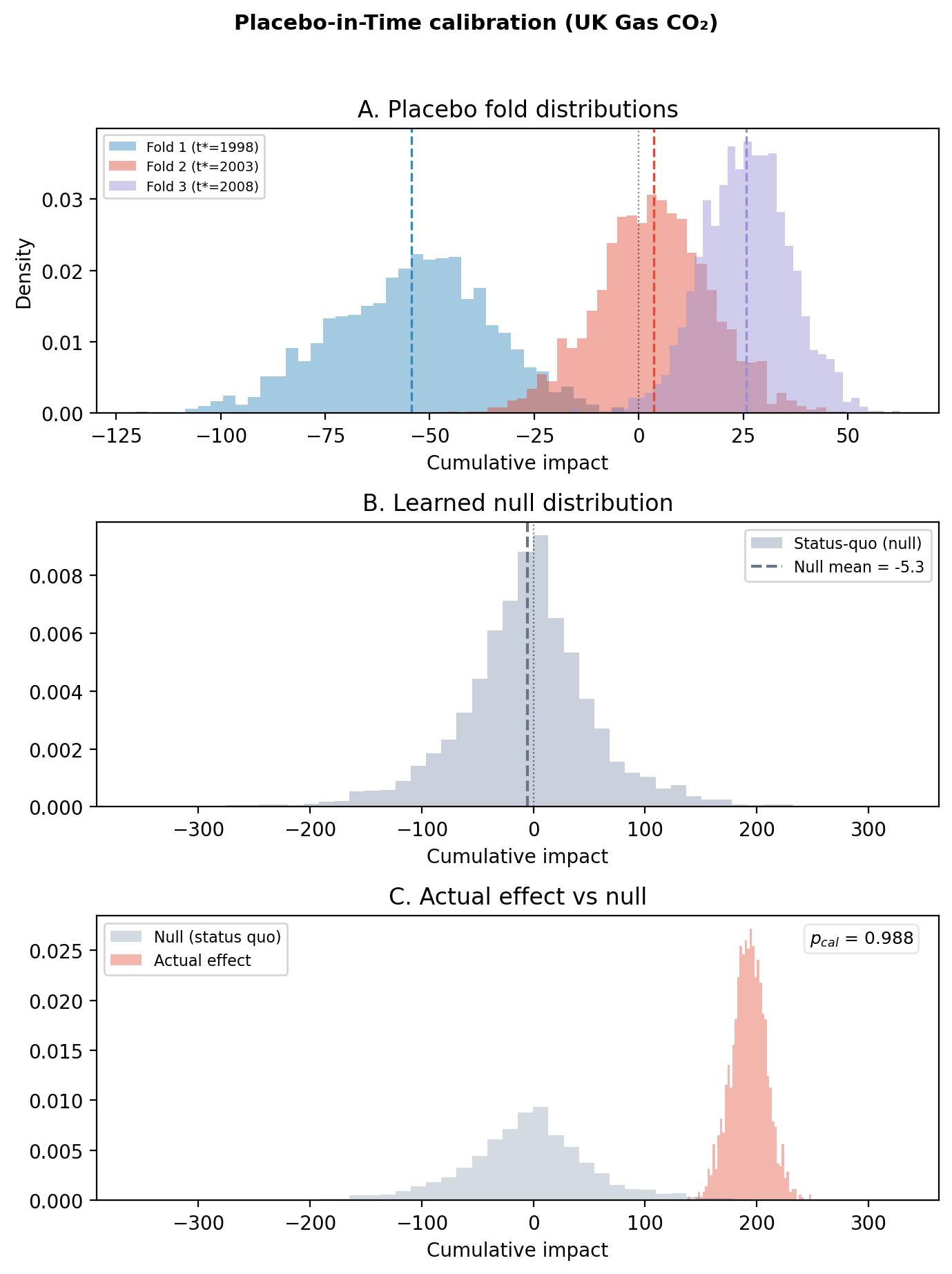
Gas tells a much cleaner story than coal did. The actual cumulative effect is +192 MtCO₂ with a placebo null about five times tighter (\(\tau_{\text{het}} \approx 50\) vs ~250 for coal), so the printed P(actual outside null) ≈ 0.99 clears the 0.95 threshold and the check returns SUPPORTED. Why tighter? The gas series swings less in the pre-period, so the three placebo windows produce more consistent “null effects” (the panel-A fold means stay within roughly ±50 MtCO₂), which shrinks the structural-noise spread the null is built from.

The energy system didn’t shrink; it reorganised. Coal’s share was absorbed by gas-fired generation, exactly as the policy intended. And crucially, this is the first piece of evidence that the coal drop wasn’t just structural noise: an unrelated outcome (gas CO₂) moved in the precise direction the mechanism predicts, with a verdict the placebo check actually backs.

Question 4: Did total CO₂ or energy demand change?

But notice the implication: if coal CO₂ went down and gas CO₂ went up, the net effect on total CO₂ may be smaller than either component alone. The policy didn’t eliminate emissions; it shifted them toward a less carbon-intensive fuel. That is the boundary check our table promised: if total CO₂ or energy demand also moved in suspicious ways, the coal story would need a more careful retelling.

Did total CO₂ change?

If the CPF mostly reshuffled emissions from coal to gas, total CO₂ might show a more modest break, or none at all. This would not mean the policy failed; it would mean its first-order effect was fuel switching.

result_pit_co2 = cp.Pipeline(
    data=df_uk[["co2"]],
    steps=[
        cp.EstimateEffect(
            method=cp.InterruptedTimeSeries,
            treatment_time=treatment_time,
            formula="co2 ~ 1",
            model=its_model(),
        ),
        cp.SensitivityAnalysis(
            checks=[
                cp.checks.PlaceboInTime(
                    n_folds=3,
                    selection_method="random",
                    min_gap=2,
                    random_seed=42,
                ),
            ]
        ),
    ],
).run()

Show code cell output Hide code cell output

Initializing NUTS using jitter+adapt_diag...
Multiprocess sampling (4 chains in 4 jobs)
NUTS: [fourier_beta, delta, beta, sigma]

Sampling 4 chains for 1_000 tune and 400 draw iterations (4_000 + 1_600 draws total) took 251 seconds.
The effective sample size per chain is smaller than 100 for some parameters.  A higher number is needed for reliable rhat and ess computation. See https://arxiv.org/abs/1903.08008 for details
Sampling: [beta, delta, fourier_beta, sigma, y_hat]
Sampling: [y_hat]

Sampling: [y_hat]
Sampling: [y_hat]
Sampling: [y_hat]
Initializing NUTS using jitter+adapt_diag...
Multiprocess sampling (4 chains in 4 jobs)
NUTS: [fourier_beta, delta, beta, sigma]

Sampling 4 chains for 1_000 tune and 400 draw iterations (4_000 + 1_600 draws total) took 165 seconds.
There was 1 divergence after tuning. Increase `target_accept` or reparameterize.
The rhat statistic is larger than 1.01 for some parameters. This indicates problems during sampling. See https://arxiv.org/abs/1903.08008 for details
The effective sample size per chain is smaller than 100 for some parameters.  A higher number is needed for reliable rhat and ess computation. See https://arxiv.org/abs/1903.08008 for details
Sampling: [beta, delta, fourier_beta, sigma, y_hat]
Sampling: [y_hat]

Sampling: [y_hat]
Sampling: [y_hat]
Sampling: [y_hat]
Initializing NUTS using jitter+adapt_diag...
Multiprocess sampling (4 chains in 4 jobs)
NUTS: [fourier_beta, delta, beta, sigma]

Sampling 4 chains for 1_000 tune and 400 draw iterations (4_000 + 1_600 draws total) took 258 seconds.
The rhat statistic is larger than 1.01 for some parameters. This indicates problems during sampling. See https://arxiv.org/abs/1903.08008 for details
Sampling: [beta, delta, fourier_beta, sigma, y_hat]
Sampling: [y_hat]

Sampling: [y_hat]
Sampling: [y_hat]
Sampling: [y_hat]
Initializing NUTS using jitter+adapt_diag...
Multiprocess sampling (4 chains in 4 jobs)
NUTS: [fourier_beta, delta, beta, sigma]

Sampling 4 chains for 1_000 tune and 400 draw iterations (4_000 + 1_600 draws total) took 572 seconds.
Sampling: [beta, delta, fourier_beta, sigma, y_hat]
Sampling: [y_hat]

Sampling: [y_hat]
Sampling: [y_hat]
Sampling: [y_hat]
Initializing NUTS using jitter+adapt_diag...
Multiprocess sampling (4 chains in 4 jobs)
NUTS: [mu_status_quo, tau_status_quo, fold_z]

Sampling 4 chains for 1_000 tune and 1_000 draw iterations (4_000 + 4_000 draws total) took 5 seconds.
Sampling: [theta_new]

pit_check_co2 = result_pit_co2.sensitivity_results[0]
print(pit_check_co2.text)

Placebo-in-time analysis: 3 of 3 folds completed.
Hierarchical status-quo model: mu=12.04, tau=360.57.
Actual cumulative impact: -45.66. P(actual outside null) = 0.098.
NOT SUPPORTED — actual effect is within the null distribution.
Fold 1: pseudo treatment at 1998-01-01 00:00:00 — mean=285.79, sd=25.38
Fold 2: pseudo treatment at 2003-01-01 00:00:00 — mean=19.44, sd=11.61
Fold 3: pseudo treatment at 2008-01-01 00:00:00 — mean=-261.35, sd=14.54

Show code cell source Hide code cell source

plot_placebo_calibration(
    pit_check=pit_check_co2,
    original_result=result_pit_co2.experiment,
    title="Placebo-in-Time calibration (UK Total CO₂)",
)

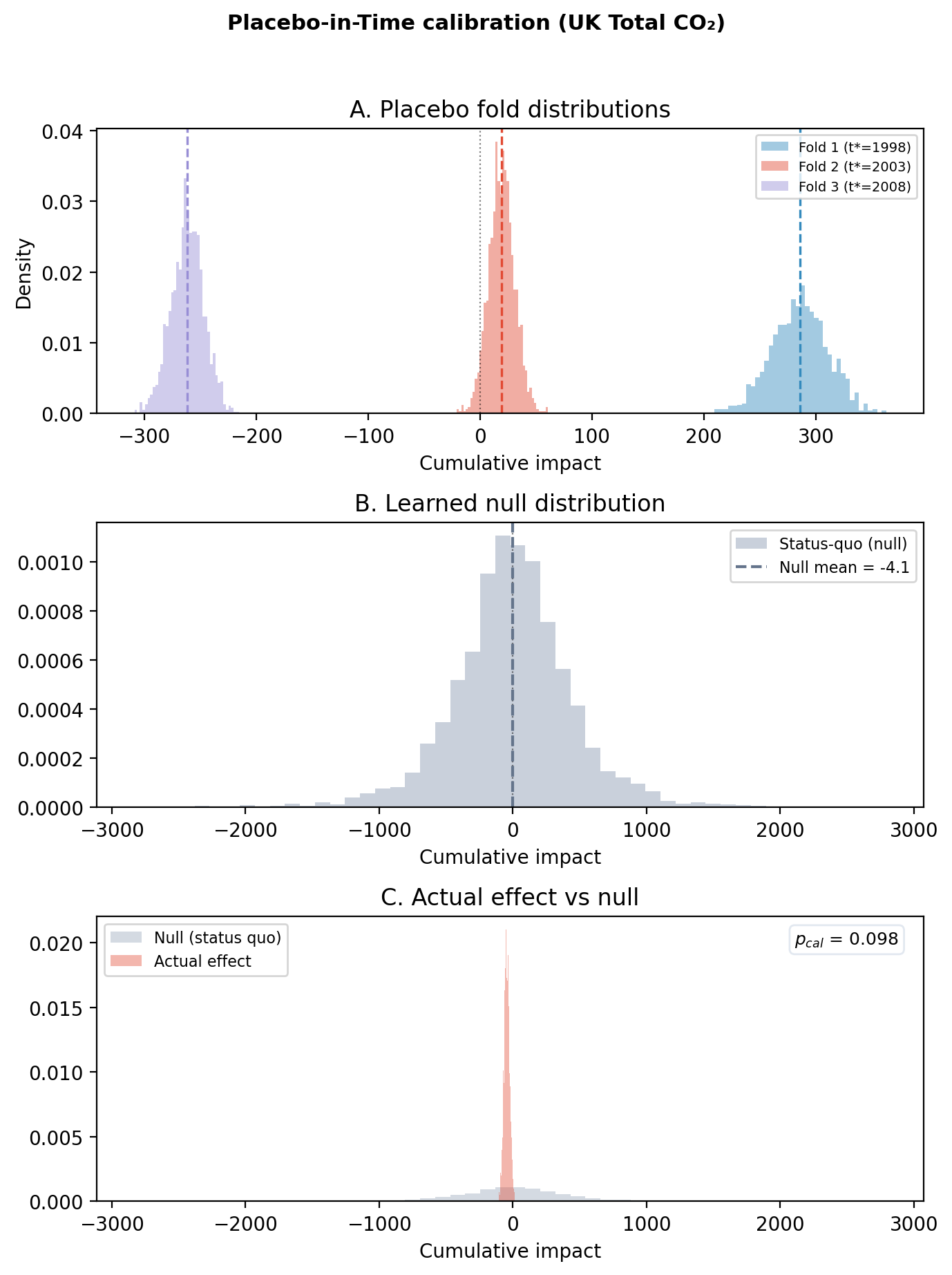
This is exactly what we predicted. The actual cumulative effect on total CO₂ is small and the placebo null fully absorbs it: the printed P(actual outside null) is well below 0.95 and the check returns NOT SUPPORTED. Here NOT SUPPORTED is the right answer: it means total CO₂ moved within what this model would have reported even if nothing had happened. That is exactly the signature of partial substitution: the CPF killed coal, gas absorbed most of the slack, and the net carbon reduction is much smaller than the coal-specific one.

This result strengthens our causal claim about coal in two ways. First, if the coal drop had been a data artefact or a recession effect, total CO₂ should have moved by a similar amount; it didn’t. Second, the contrast between Question 3 (gas SUPPORTED, +192 MtCO₂) and Question 4 (total NOT SUPPORTED, small effect) is exactly what a fuel-switching mechanism predicts and is hard to fake with model error alone.

Did energy demand change?

The final check. A skeptic’s strongest objection: “Maybe the UK economy crashed in 2013, and the drop in CO₂ was just a byproduct of a recession.”

If that were true, the relationship between energy use and economic output would break. We can test this by looking at Energy Intensity (energy_per_gdp) — how much energy it takes to generate one dollar of GDP.

The Carbon Price Floor was designed to clean up the supply side (taxing dirty fuel), not to destroy the demand side (economic output). If the policy worked as intended, the UK economy should have continued generating wealth at its historical rate of energy efficiency. If the energy_per_gdp trend remains perfectly stable through 2013, the recession story collapses.

sampler_kwargs = {
    "nuts_sampler": "nutpie",
    "nuts_sampler_kwargs": {"backend": "jax", "gradient_backend": "jax"},
    "target_accept": 0.94,
}


def states_space_model():
    """Fresh StateSpaceTimeSeries model (single-use)."""
    return cp.pymc_models.StateSpaceTimeSeries(
        level_order=3,
        seasonal_length=2,
        sample_kwargs=sampler_kwargs,
        mode="FAST_COMPILE",
    )


# Calculate GDP per capita
df_uk_epc = df_uk.dropna(subset=["energy_per_gdp"]).copy()

result_epc = cp.InterruptedTimeSeries(
    data=df_uk_epc[["energy_per_gdp"]],
    treatment_time=treatment_time,
    formula="energy_per_gdp ~ 1",
    model=states_space_model(),
)

Show code cell output Hide code cell output

                                Model Requirements                                
                                                                                  
  Variable              Shape    Constraints                          Dimensions  
 ──────────────────────────────────────────────────────────────────────────────── 
  initial_level_trend   (3,)                              ('state_level_trend',)  
  sigma_level_trend     (3,)     Positive                 ('shock_level_trend',)  
  params_freq           (1,)                                     ('state_freq',)  
  sigma_freq            ()       Positive                                   None  
  P0                    (5, 5)   Positive semi-definite   ('state', 'state_aux')  
                                                                                  
   These parameters should be assigned priors inside a PyMC model block before    
                    calling the build_statespace_graph method.                    

Sampler Progress

Total Chains: 4

Active Chains: 0

Finished Chains: 4

Sampling for now

Estimated Time to Completion: now

Progress	Draws	Divergences	Step Size	Gradients/Draw
	2000	2	0.34	15
	2000	8	0.35	15
	2000	1	0.33	15
	2000	3	0.38	15

Sampling: [obs]

Sampling: [filtered_posterior, filtered_posterior_observed, predicted_posterior, predicted_posterior_observed, smoothed_posterior, smoothed_posterior_observed]

Sampling: [forecast_combined]

Show code cell source Hide code cell source

fig, axes = result_epc.plot(show=False)
axes[0].set_title("ITS (State-Space) — UK Energy per GDP (Falsification)")
plt.tight_layout()
plt.show()

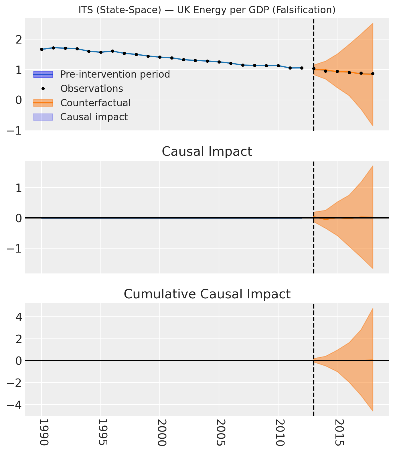
Energy per GDP shows no meaningful break at 2013. The actual trajectory hugs the counterfactual. People kept generating roughly the same amount of economic output per unit of energy; they just stopped getting that energy from coal.

Assembling the case

We did not prove that the Carbon Price Floor caused the decline in coal CO₂. Proof is not available in observational data. What we did is accumulate four pieces of evidence, each small, each pointing in the same direction:

Step	What we found	Placebo verdict	What it rules out
Coal CO₂ collapsed	Large negative effect (~-416 MtCO₂), but a wide structural null	NOT SUPPORTED (\(p_{\text{cal}} \approx 0.84\)) on its own	Pure random fluctuation, but not yet structural noise — needs corroboration
Gas CO₂ rose	Clear substitution toward gas (~+192 MtCO₂, tighter null)	SUPPORTED (\(p_{\text{cal}} \approx 0.99\))	A general decline in all fuels, or coal being explained by something other than substitution
Total CO₂ effect is weaker	Small effect absorbed by the null	NOT SUPPORTED (and that’s the prediction)	Data error or recession that would push all CO₂ down equally
Energy demand stayed flat	No break in energy_per_gdp at 2013	(qualitative)	Recession or demand shock

No single finding is conclusive, and the coal-CO₂ placebo, taken alone, does not even clear the 0.95 SUPPORTED bar. That is the point. The four pieces together tell a coherent story the individual checks cannot tell: the Carbon Price Floor made coal uncompetitive, energy producers switched to gas (SUPPORTED), coal CO₂ collapsed (large effect but inside a wide structural null), total CO₂ fell modestly (consistent with substitution rather than elimination), and energy demand was unaffected (no recession). Each line in the table closes off a different alternative explanation; the case is the pile, not any one entry.