Regression kink design with pymc models#
import arviz as az
import matplotlib.pyplot as plt
import numpy as np
import pandas as pd

import causalpy as cp
%load_ext autoreload
%autoreload 2
%config InlineBackend.figure_format = 'retina'
seed = 42
rng = np.random.default_rng(seed)
The Regression kink design should be analysed by a piecewise continuous function. That is:
We want a function which can capture the data to the left and to the right of the kink point.
We want a piecewise function with one breakpoint or kink point
The function should be continuous at the kink point
An example of such a function would be a piecewise continuous polynomial:
Where:
\(\beta\)’s are the unknown parameters,
\(x\) is the running variable,
\(t\) is an indicator variable which is \(1\) if \(x \geq k\), and \(0\) otherwise,
\(k\) is the value of \(x\) at the kink point.
We can visualise what these functions look like by plotting a number of them with randomly chosen \(\beta\) coefficients, but all with a kink point at \(0.5\).
def f(x, beta, kink):
    return (
        beta[0]
        + beta[1] * x
        + beta[2] * x**2
        + beta[3] * (x - kink) * (x >= kink)
        + beta[4] * (x - kink) ** 2 * (x >= kink)
    )


def gradient_change(beta, kink, epsilon=0.01):
    gradient_left = (f(kink, beta, kink) - f(kink - epsilon, beta, kink)) / epsilon
    gradient_right = (f(kink + epsilon, beta, kink) - f(kink, beta, kink)) / epsilon
    gradient_change = gradient_right - gradient_left
    return gradient_change


x = np.linspace(-1, 1, 1000)
kink = 0.5
cols = 5

fig, ax = plt.subplots(2, cols, sharex=True, sharey=True, figsize=(15, 5))

for col in range(cols):
    beta = rng.random(5)
    ax[0, col].plot(x, f(x, beta, kink), lw=3)
    ax[1, col].plot(x, np.gradient(f(x, beta, kink), x), lw=3)
    ax[0, col].set(title=f"Random  {col + 1}")
    ax[1, col].set(xlabel="x")

ax[0, 0].set(ylabel="$y = f(x)$")
ax[1, 0].set(ylabel=r"$\frac{dy}{dx}$");
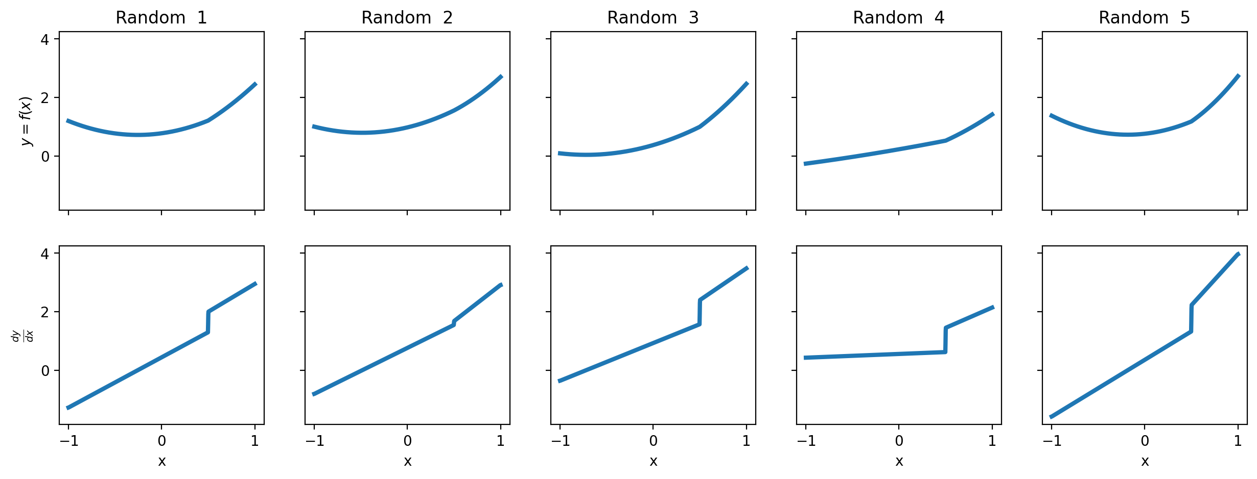
The idea of regression kink analysis is to fit a suitable function to data and to estimate whether there is a change in the gradient of the function at the kink point.
Below we will generate a number of datasets and run through how to conduct the regression kink analysis. We will use a function to generate simulated datasets with the properties we want.
def generate_data(beta, kink, sigma=0.05, N=50):
    if beta is None:
        beta = rng.random(5)
    x = rng.uniform(-1, 1, N)
    y = f(x, beta, kink) + rng.normal(0, sigma, N)
    df = pd.DataFrame({"x": x, "y": y, "treated": x >= kink})
    return df
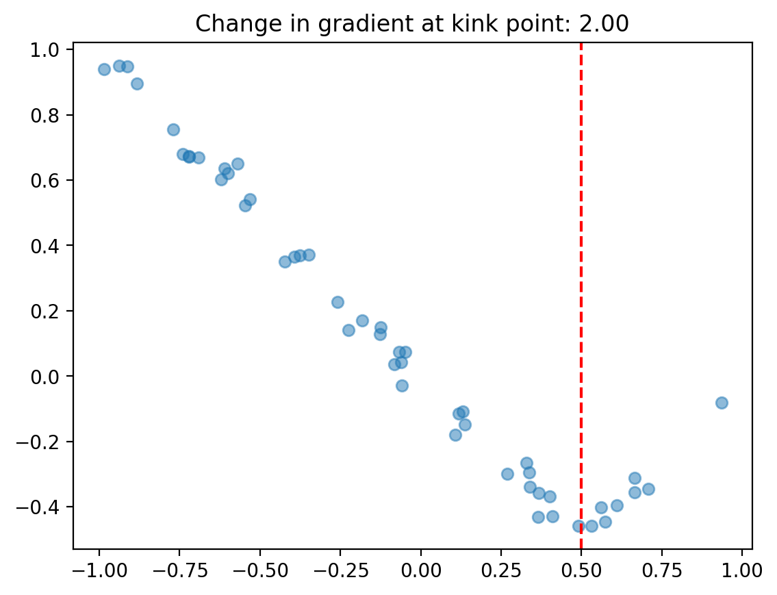
Example 1 - continuous piecewise linear function#
In this example we’ll stick to a simple continuous piecewise function.
kink = 0.5
# linear function with gradient change of 2 at kink point
beta = [0, -1, 0, 2, 0]
sigma = 0.05
df = generate_data(beta, kink, sigma=sigma)

fig, ax = plt.subplots()
ax.scatter(df["x"], df["y"], alpha=0.5)
ax.axvline(kink, color="red", linestyle="--")
ax.set(title=f"Change in gradient at kink point: {gradient_change(beta, kink):.2f}");
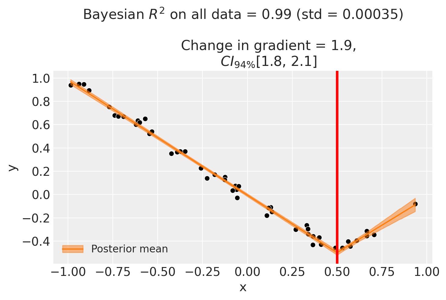
We can use the regular cp.pymc_models.LinearRegression model and enforce the continuous piecewise nature by cleverly specifying a design matrix via the formula input.
In this example, setting the formula to "y ~ 1 + x + I((x-0.5)*treated)" (where the 0.5 is the kink point) equates to the following model:
Note
The change in gradient either side of the kink point is evaluated numerically. The epsilon parameter determines the distance either side of the kink point that is used in this change in gradient calculation.
result1 = cp.RegressionKink(
    df,
    formula=f"y ~ 1 + x + I((x-{kink})*treated)",
    model=cp.pymc_models.LinearRegression(sample_kwargs={"random_seed": seed}),
    kink_point=kink,
    epsilon=0.1,
)

fig, ax = result1.plot()
Initializing NUTS using jitter+adapt_diag...
Multiprocess sampling (4 chains in 4 jobs)
NUTS: [beta, y_hat_sigma]
Sampling 4 chains for 1_000 tune and 1_000 draw iterations (4_000 + 4_000 draws total) took 1 seconds.
Sampling: [beta, y_hat, y_hat_sigma]
Sampling: [y_hat]
Sampling: [y_hat]
Sampling: [y_hat]
Sampling: [y_hat]
If you want to plot the posterior distribution of the inferred gradient change, you can do it as follows.
ax = az.plot_posterior(result1.gradient_change, ref_val=gradient_change(beta, kink))
ax.set(title="Gradient change");
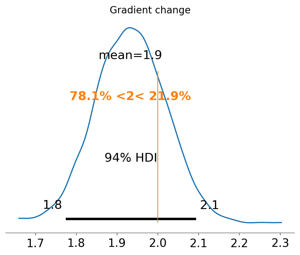
We know that the correct gradient change is 2, and that we have correctly recovered it as the posterior distribution is centred around 2.
We can also ask for summary information:
result1.summary()
        ================================Regression Kink=================================
        Formula: y ~ 1 + x + I((x-0.5)*treated)
        Running variable: x
        Kink point on running variable: 0.5

        Results:
        Change in slope at kink point = 1.9

Model coefficients:
    Intercept               -0.0058, 94% HDI [-0.018, 0.0059]
    x                       -0.99, 94% HDI [-1, -0.96]
    I((x - 0.5) * treated)  1.9, 94% HDI [1.8, 2.1]
    y_hat_sigma             0.039, 94% HDI [0.032, 0.047]
For Regression Kink, the effect_summary() method provides a decision-ready report of the change in gradient (slope) at the kink point:
stats1 = result1.effect_summary()
stats1.table
| mean | median | hdi_lower | hdi_upper | p_gt_0 | |
|---|---|---|---|---|---|
| gradient_change | 1.932667 | 1.931843 | 1.771899 | 2.107181 | 1.0 |
Example 2 - continuous piecewise polynomial function#
Now we’ll introduce some nonlinearity into the mix.
In this example, we’re going to have a 2nd order polynomial on either side of the kink point. So the model can be defined as:
While it’s a bit verbose, we can implement this in a patsy formula as so:
y ~ 1 + x + np.power(x, 2) + I((x-0.5)*treated) + I(np.power((x-0.5), 2)*treated)
where the 0.5 is the kink point.
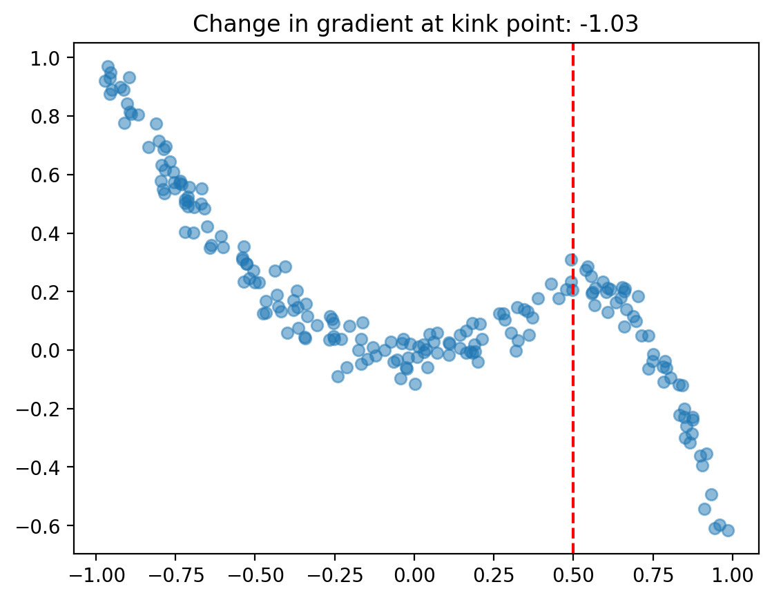
kink = 0.5
# quadratic function going from 1*x^2 on the left of the kink point, to 1*x^2 -
# 1*(x-kink) - 5*(x-kink)^2 to the right of the kink point
beta = [0, 0, 1, -1, -5]
df = generate_data(beta, kink, N=200, sigma=sigma)

fig, ax = plt.subplots()
ax.scatter(df["x"], df["y"], alpha=0.5)
ax.axvline(kink, color="red", linestyle="--")
ax.set(title=f"Change in gradient at kink point: {gradient_change(beta, kink):.2f}");
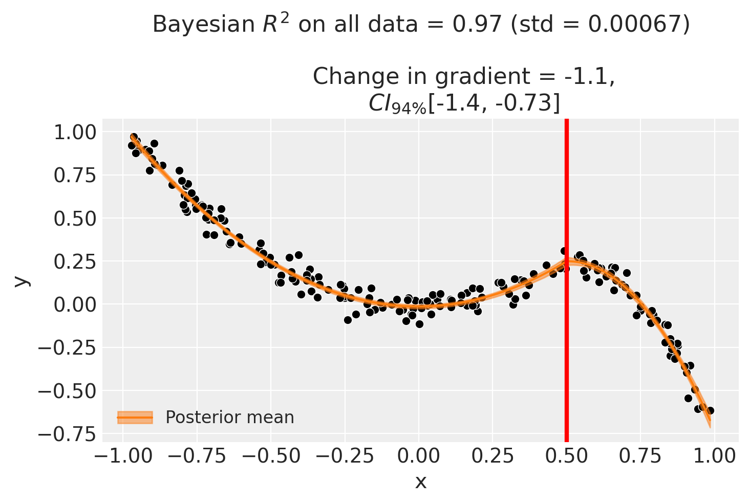
formula = f"y ~ 1 + x + np.power(x, 2) + I((x-{kink})*treated) + I(np.power(x-{kink}, 2)*treated)"
result2 = cp.RegressionKink(
df,
formula=formula,
model=cp.pymc_models.LinearRegression(sample_kwargs={"random_seed": seed}),
kink_point=kink,
epsilon=0.01,
)
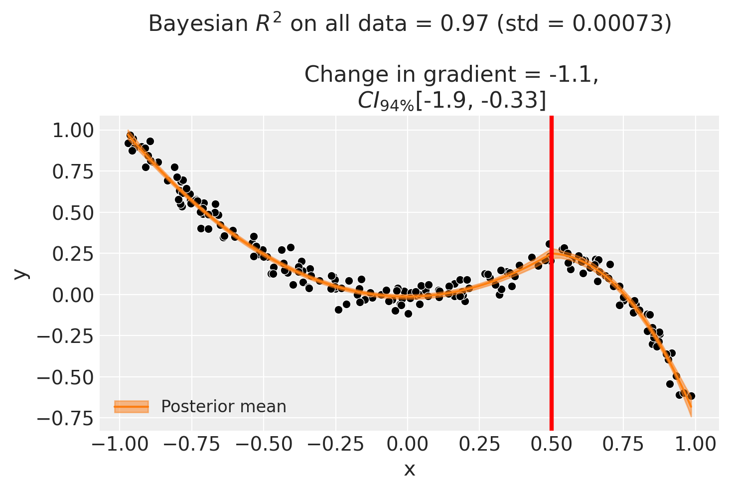
fig, ax = result2.plot()
Initializing NUTS using jitter+adapt_diag...
Multiprocess sampling (4 chains in 4 jobs)
NUTS: [beta, y_hat_sigma]
Sampling 4 chains for 1_000 tune and 1_000 draw iterations (4_000 + 4_000 draws total) took 1 seconds.
Sampling: [beta, y_hat, y_hat_sigma]
Sampling: [y_hat]
Sampling: [y_hat]
Sampling: [y_hat]
Sampling: [y_hat]
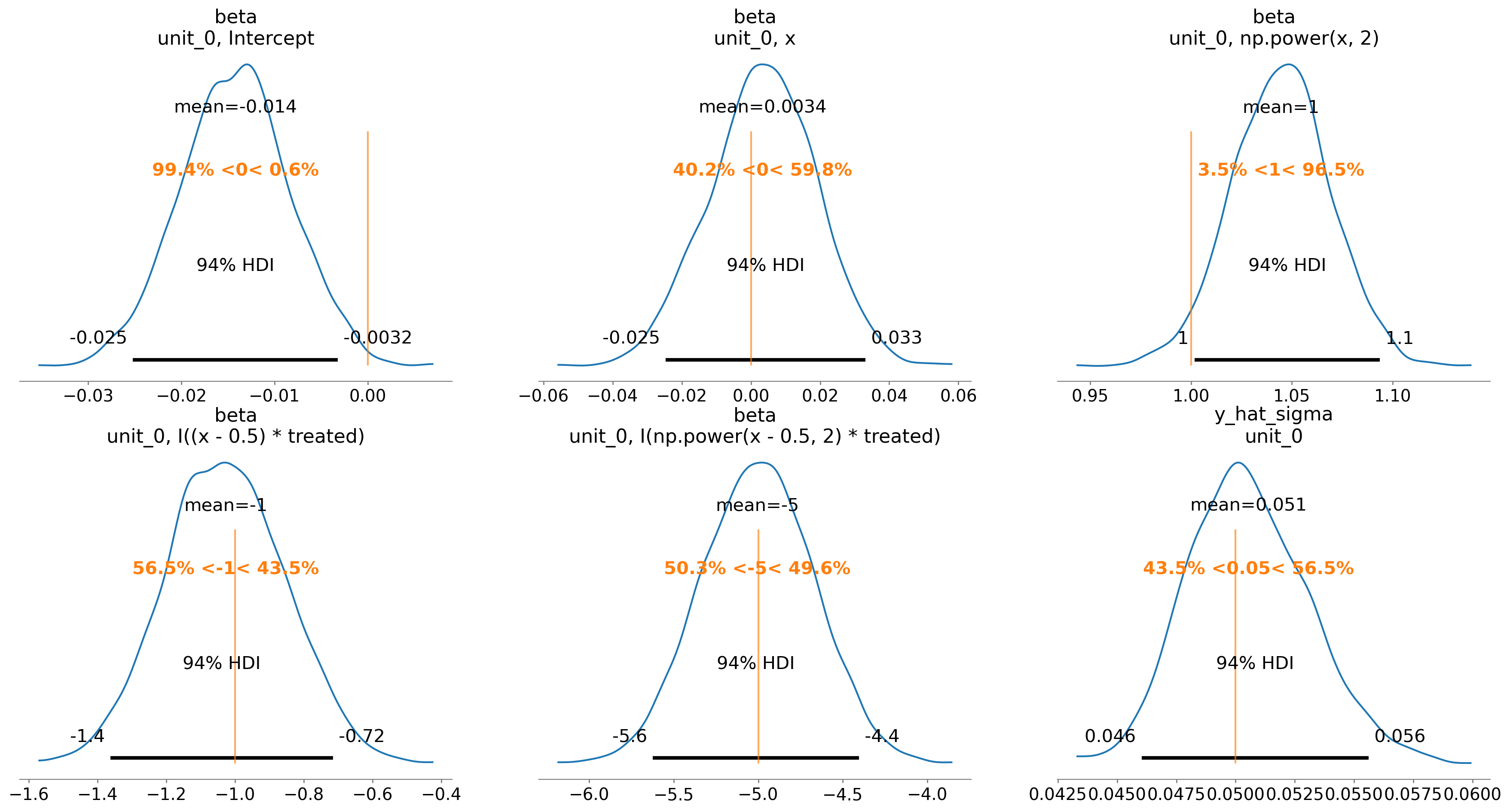
We can also evaluate the posterior distribution of the parameters and see how they match up with the true values.
ax = az.plot_posterior(
    result2.idata, var_names=["beta", "y_hat_sigma"], ref_val=beta + [sigma]
)
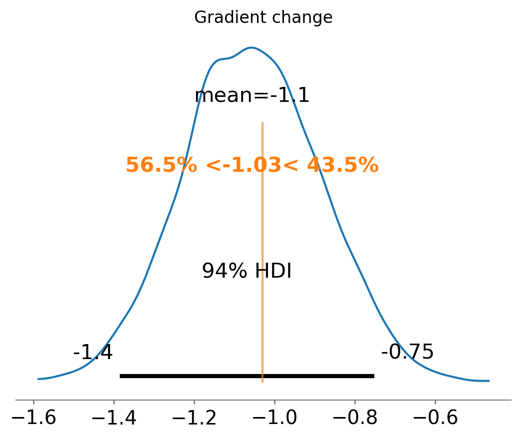
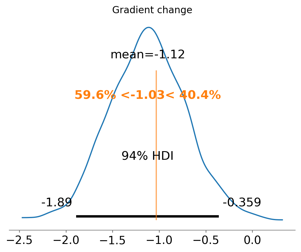
Finally, we can see that we have also done a good job at recovering the true gradient change.
ax = az.plot_posterior(result2.gradient_change, ref_val=gradient_change(beta, kink))
ax.set(title="Gradient change");
And the effect summary for the polynomial model:
stats2 = result2.effect_summary()
stats2.table
| mean | median | hdi_lower | hdi_upper | p_gt_0 | |
|---|---|---|---|---|---|
| gradient_change | -1.056407 | -1.06007 | -1.385243 | -0.723697 | 0.0 |
Example 3 - basis spline model#
As a final example to demonstrate that we need not be constrained to polynomial functions, we can use a basis spline model. This takes advantage of the capability of patsy to generate design matrices with basis splines. Note that we will use the same simulated dataset as the previous example.
result3 = cp.RegressionKink(
    df,
    formula=f"y ~ 1 + bs(x, df=3) + bs(I(x-{kink})*treated, df=3)",
    model=cp.pymc_models.LinearRegression(sample_kwargs={"random_seed": seed}),
    kink_point=kink,
)

result3.plot();
Initializing NUTS using jitter+adapt_diag...
Multiprocess sampling (4 chains in 4 jobs)
NUTS: [beta, y_hat_sigma]
Sampling 4 chains for 1_000 tune and 1_000 draw iterations (4_000 + 4_000 draws total) took 2 seconds.
Sampling: [beta, y_hat, y_hat_sigma]
Sampling: [y_hat]
Sampling: [y_hat]
Sampling: [y_hat]
Sampling: [y_hat]
ax = az.plot_posterior(
    result3.gradient_change, ref_val=gradient_change(beta, kink), round_to=3
)
ax.set(title="Gradient change");
For the basis spline model:
stats3 = result3.effect_summary()
stats3.table
| mean | median | hdi_lower | hdi_upper | p_gt_0 | |
|---|---|---|---|---|---|
| gradient_change | -1.123113 | -1.122874 | -1.892855 | -0.292991 | 0.004 |
Using a bandwidth#
If we don’t want to fit on all the data available, we can use the bandwidth kwarg. This will only fit the model to data within a certain bandwidth of the kink point. If \(x\) is the running variable, then the model will only be fitted to data where \(threshold - bandwidth \le x \le threshold + bandwidth\).
formula = f"y ~ 1 + x + np.power(x, 2) + I((x-{kink})*treated) + I(np.power(x-{kink}, 2)*treated)"

result4 = cp.RegressionKink(
    df,
    formula=formula,
    model=cp.pymc_models.LinearRegression(sample_kwargs={"random_seed": seed}),
    kink_point=kink,
    epsilon=0.01,
    bandwidth=0.4,
)

fig, ax = result4.plot()
Initializing NUTS using jitter+adapt_diag...
Multiprocess sampling (4 chains in 4 jobs)
NUTS: [beta, y_hat_sigma]
Sampling 4 chains for 1_000 tune and 1_000 draw iterations (4_000 + 4_000 draws total) took 7 seconds.
There were 27 divergences after tuning. Increase `target_accept` or reparameterize.
Sampling: [beta, y_hat, y_hat_sigma]
Sampling: [y_hat]
Sampling: [y_hat]
Sampling: [y_hat]
Sampling: [y_hat]
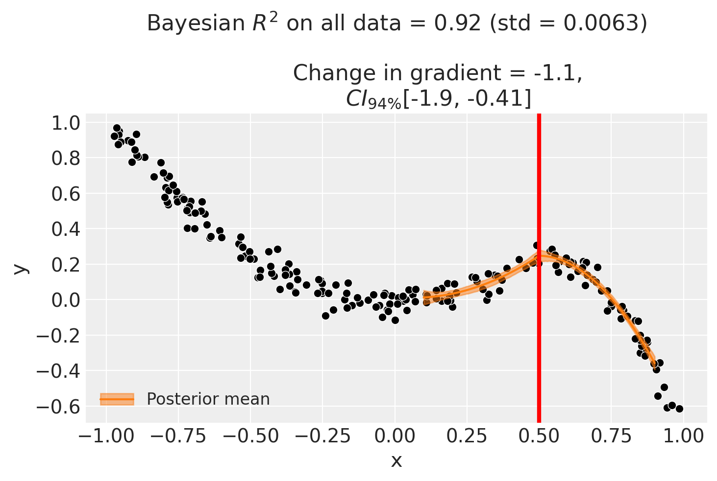
And for the bandwidth-restricted model:
stats4 = result4.effect_summary()
stats4.table
| mean | median | hdi_lower | hdi_upper | p_gt_0 | |
|---|---|---|---|---|---|
| gradient_change | -1.147603 | -1.14399 | -1.929114 | -0.383215 | 0.0025 |
Sensitivity analysis#
Bandwidth sensitivity#
As with regression discontinuity, the regression kink design involves a bias–variance trade-off in the choice of bandwidth. A narrow bandwidth focuses on observations close to the kink point, reducing bias from functional-form mis-specification but increasing variance. A wide bandwidth includes more data but risks capturing curvature that does not reflect the true kink effect [Imbens and Lemieux, 2008].
BandwidthSensitivity refits the model at several bandwidths (0.1, 0.25, 0.5, and 1.0) and reports the estimated change in gradient at each. If the estimate is stable across bandwidths, this provides evidence that the result is not driven by a particular bandwidth choice.
Interpreting the output. The report shows a table with the effect estimate at each bandwidth. Look for consistency: if the estimates vary substantially, this suggests the result is sensitive to the amount of data used, which may indicate model mis-specification near the kink point.
kink_sensitivity = 0.5
beta_sensitivity = [0, -1, 0, 2, 0]
df_sensitivity = generate_data(beta_sensitivity, kink_sensitivity, sigma=0.05)

sensitivity_result = cp.Pipeline(
    data=df_sensitivity,
    steps=[
        cp.EstimateEffect(
            method=cp.RegressionKink,
            formula=f"y ~ 1 + x + I((x-{kink_sensitivity})*treated)",
            model=cp.pymc_models.LinearRegression(sample_kwargs={"random_seed": seed}),
            kink_point=kink_sensitivity,
            epsilon=0.1,
        ),
        cp.SensitivityAnalysis(
            checks=[
                cp.checks.BandwidthSensitivity(bandwidths=[0.1, 0.25, 0.5, 1.0]),
            ],
        ),
        cp.GenerateReport(include_plots=True),
    ],
).run()

for cr in sensitivity_result.sensitivity_results:
    print(cr.text)
Initializing NUTS using jitter+adapt_diag...
Multiprocess sampling (4 chains in 4 jobs)
NUTS: [beta, y_hat_sigma]
Sampling 4 chains for 1_000 tune and 1_000 draw iterations (4_000 + 4_000 draws total) took 1 seconds.
Sampling: [beta, y_hat, y_hat_sigma]
Sampling: [y_hat]
Sampling: [y_hat]
Sampling: [y_hat]
Sampling: [y_hat]
/Users/benjamv/git/CausalPy/causalpy/experiments/regression_kink.py:90: UserWarning: Choice of bandwidth parameter has lead to only 3 remaining datapoints. Consider increasing the bandwidth parameter.
  self._build_design_matrices()
Initializing NUTS using jitter+adapt_diag...
Multiprocess sampling (4 chains in 4 jobs)
NUTS: [beta, y_hat_sigma]
Sampling 4 chains for 1_000 tune and 1_000 draw iterations (4_000 + 4_000 draws total) took 8 seconds.
There were 326 divergences after tuning. Increase `target_accept` or reparameterize.
The rhat statistic is larger than 1.01 for some parameters. This indicates problems during sampling. See https://arxiv.org/abs/1903.08008 for details
The effective sample size per chain is smaller than 100 for some parameters. A higher number is needed for reliable rhat and ess computation. See https://arxiv.org/abs/1903.08008 for details
Sampling: [beta, y_hat, y_hat_sigma]
Sampling: [y_hat]
Sampling: [y_hat]
Sampling: [y_hat]
Sampling: [y_hat]
Initializing NUTS using jitter+adapt_diag...
Multiprocess sampling (4 chains in 4 jobs)
NUTS: [beta, y_hat_sigma]
Sampling 4 chains for 1_000 tune and 1_000 draw iterations (4_000 + 4_000 draws total) took 1 seconds.
There were 77 divergences after tuning. Increase `target_accept` or reparameterize.
The rhat statistic is larger than 1.01 for some parameters. This indicates problems during sampling. See https://arxiv.org/abs/1903.08008 for details
Sampling: [beta, y_hat, y_hat_sigma]
Sampling: [y_hat]
Sampling: [y_hat]
Sampling: [y_hat]
Sampling: [y_hat]
Initializing NUTS using jitter+adapt_diag...
Multiprocess sampling (4 chains in 4 jobs)
NUTS: [beta, y_hat_sigma]
Sampling 4 chains for 1_000 tune and 1_000 draw iterations (4_000 + 4_000 draws total) took 1 seconds.
There was 1 divergence after tuning. Increase `target_accept` or reparameterize.
Sampling: [beta, y_hat, y_hat_sigma]
Sampling: [y_hat]
Sampling: [y_hat]
Sampling: [y_hat]
Sampling: [y_hat]
Initializing NUTS using jitter+adapt_diag...
Multiprocess sampling (4 chains in 4 jobs)
NUTS: [beta, y_hat_sigma]
Sampling 4 chains for 1_000 tune and 1_000 draw iterations (4_000 + 4_000 draws total) took 1 seconds.
Sampling: [beta, y_hat, y_hat_sigma]
Sampling: [y_hat]
Sampling: [y_hat]
Sampling: [y_hat]
Sampling: [y_hat]
Bandwidth sensitivity analysis: compared 4 bandwidth values. Examine the table for consistency of effect estimates across bandwidths.
import html as html_module
import warnings

from IPython.display import HTML

with warnings.catch_warnings():
    warnings.filterwarnings(
        "ignore", "Consider using IPython.display.IFrame", UserWarning
    )
    display(
        HTML(
            f'<iframe srcdoc="{html_module.escape(sensitivity_result.report)}" '
            f'width="100%" height="600" style="border:1px solid #ccc;"></iframe>'
        )
    )