Example Interrupted Time Series (ITS) with pymc models

This notebook shows an example of using interrupted time series, where we do not have untreated control units of a similar nature to the treated unit and we just have a single time series of observations and the predictor variables are simply time and month.

import arviz as az
import pandas as pd

import causalpy as cp

WARNING (pytensor.tensor.blas): Using NumPy C-API based implementation for BLAS functions.

%load_ext autoreload
%autoreload 2
%config InlineBackend.figure_format = 'retina'
seed = 42

Interrupted Time Series (ITS) Example

Load data

df = (
    cp.load_data("its")
    .assign(date=lambda x: pd.to_datetime(x["date"]))
    .set_index("date")
)

treatment_time = pd.to_datetime("2017-01-01")
df.head()

	month	year	t	y
date
2010-01-31	1	2010	0	25.058186
2010-02-28	2	2010	1	27.189812
2010-03-31	3	2010	2	26.487551
2010-04-30	4	2010	3	31.241716
2010-05-31	5	2010	4	40.753973

Run the analysis

Note

The random_seed keyword argument for the PyMC sampler is not neccessary. We use it here so that the results are reproducible.

result = cp.pymc_experiments.InterruptedTimeSeries(
    df,
    treatment_time,
    formula="y ~ 1 + t + C(month)",
    model=cp.pymc_models.LinearRegression(sample_kwargs={"random_seed": seed}),
)

Auto-assigning NUTS sampler...
Initializing NUTS using jitter+adapt_diag...
Multiprocess sampling (4 chains in 4 jobs)
NUTS: [beta, sigma]

100.00% [8000/8000 00:02<00:00 Sampling 4 chains, 0 divergences]

Sampling 4 chains for 1_000 tune and 1_000 draw iterations (4_000 + 4_000 draws total) took 2 seconds.
Sampling: [beta, sigma, y_hat]
Sampling: [y_hat]
Sampling: [y_hat]
Sampling: [y_hat]
Sampling: [y_hat]

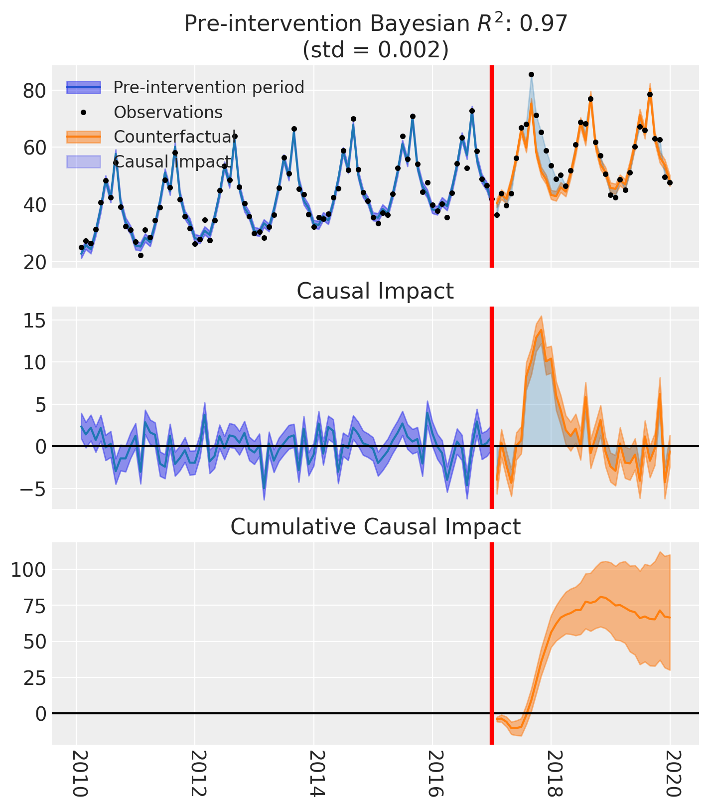
fig, ax = result.plot()

result.summary()

==================================Pre-Post Fit==================================
Formula: y ~ 1 + t + C(month)
Model coefficients:
Intercept                     23, 94% HDI [21, 24]
C(month)[T.2]                 2.8, 94% HDI [0.8, 4.8]
C(month)[T.3]                 1.1, 94% HDI [-0.93, 3.1]
C(month)[T.4]                 7.1, 94% HDI [5.1, 9.1]
C(month)[T.5]                 15, 94% HDI [13, 17]
C(month)[T.6]                 25, 94% HDI [23, 27]
C(month)[T.7]                 18, 94% HDI [16, 20]
C(month)[T.8]                 33, 94% HDI [32, 35]
C(month)[T.9]                 16, 94% HDI [14, 18]
C(month)[T.10]                9.2, 94% HDI [7.1, 11]
C(month)[T.11]                6.3, 94% HDI [4.2, 8.2]
C(month)[T.12]                0.54, 94% HDI [-1.6, 2.6]
t                             0.21, 94% HDI [0.19, 0.23]
sigma                         2, 94% HDI [1.7, 2.3]

As well as the model coefficients, we might be interested in the avarage causal impact and average cumulative causal impact.

Note

Better output for the summary statistics are in progress!

First we ask for summary statistics of the causal impact over the entire post-intervention period.

az.summary(result.post_impact.mean("obs_ind"))

	mean	sd	hdi_3%	hdi_97%	mcse_mean	mcse_sd	ess_bulk	ess_tail	r_hat
x	1.825	0.671	0.585	3.081	0.012	0.009	3108.0	3351.0	1.0

Warning

Care must be taken with the mean impact statistic. It only makes sense to use this statistic if it looks like the intervention had a lasting (and roughly constant) effect on the outcome variable. If the effect is transient, then clearly there will be a lot of post-intervention period where the impact of the intervention has ‘worn off’. If so, then it will be hard to interpret the mean impacts real meaning.

We can also ask for the summary statistics of the cumulative causal impact.

# get index of the final time point
index = result.post_impact_cumulative.obs_ind.max()
# grab the posterior distribution of the cumulative impact at this final time point
last_cumulative_estimate = result.post_impact_cumulative.sel({"obs_ind": index})
# get summary stats
az.summary(last_cumulative_estimate)

	mean	sd	hdi_3%	hdi_97%	mcse_mean	mcse_sd	ess_bulk	ess_tail	r_hat
x	65.705	24.14	21.061	110.909	0.434	0.307	3108.0	3351.0	1.0